Chapter 8.A – Functional Form 1: Linearity

All of the econometric models discussed up to this point have involved a linear relationship between a dependent variable and a set of independent variables. Anyone who has completed one or more courses in introductory economics, however, will recall seeing many graphs containing nonlinear relationships. Since many economic relationships are expected to be nonlinear, the linearity assumption seems somewhat restrictive. In this chapter, however, it will be shown that the linearity assumption is less restrictive than it initially appears.

8.1 Linearity

When the classical regression model was defined in Chapter 6, it was assumed that the regression equation could be expressed as a linear relationship, as in the simple demand equation given by:

\begin{equation}Q_{t}^{d}=\beta_{0}+\beta_{1}\text{Price}_{t}+\beta_{2}\text{Income}_{t}+u_{t} \tag{8.1} \end{equation}

where:

• [latex]Q_{t}^{d}[/latex] = quantity of a good demanded at time [latex]t[/latex]
• Price[latex]_{t}[/latex] = price of this good at time [latex]t[/latex]
• Income[latex]_{t}[/latex] = consumer income at time [latex]t[/latex]
• [latex]u_{t}[/latex] = random error term at time [latex]t[/latex]

Equation 8.1 states that the quantity demanded for a good is a linear function of price and income. More generally, a linear regression equation involving a dependent variable ([latex]Y[/latex]) and [latex]k[/latex] independent variables ([latex]X_{j}[/latex]) can be expressed as:

[latex]Y_{i}=\beta _{0}+\beta _{1}X_{1i}+\beta _{2}X_{2i}+\ldots +\beta _{k}X_{ki}+u_{i} \tag{8.2}[/latex]

Quite often, however, econometricians wish to work with models in which there is a nonlinear relationship between a dependent variable and one or more independent variables. For example, consider the regression model given by:

[latex]Y_{i}=\beta _{0}+\beta _{1}X_{i}+\beta _{2}X_{i}^{2}+u_{i} \tag{8.3}[/latex]

This model involves a nonlinear relationship between the dependent variable [latex]Y[/latex] and the independent variable [latex]X[/latex]. Fortunately, however, the model appearing in equation 8.3 (and many other nonlinear models) may be converted to a linear form by a suitable redefinition of variables. In this example, a new variable, [latex]Z_{j}[/latex], may be defined as:

[latex]Z_{j}=X_{j}^{2} \tag{8.4}[/latex]

Using this definition, equation 8.3 may be rewritten as:

[latex]Y_{i}=\beta _{0}+\beta _{1}X_{i}+\beta _{2}Z_{i}+u_{i} \tag{8.5}[/latex]

Equation 8.5 involves a linear relationship between the dependent variable and the independent variables [latex]X[/latex] and [latex]Z[/latex]. Thus, by suitably defining a new variable ([latex]Z[/latex]), a nonlinear model has been converted into the linear model appearing in equation 8.5. The parameters of equation 8.5 can be estimated using OLS estimation techniques (assuming that all of the other assumptions of the classical regression model are satisfied). These estimated intercept and slope terms serve as estimates of the parameters of the original model (equation 8.4).

In general, if an econometric model can be expressed in the form:

[latex]Y_{i}=\beta _{0}+\beta _{1}f_{1}\left( X_{1i},X_{2i},\ldots ,X_{mi}\right) +\beta _{2}f_{2}\left( X_{1i},X_{2i},\ldots ,X_{mi}\right) \tag{8.6}[/latex]

[latex]+\ldots +\beta _{k}f_{k}\left( X_{1i},X_{2i},\ldots ,X_{mi}\right) +u_{i} [/latex]

then it is always possible to rewrite the equation in the linear form:

[latex]Y_{i}=\beta _{0}+\beta _{1}\tilde{X}_{1i}+\beta _{2}\tilde{X}_{2i}+\ldots +\beta _{k}\tilde{X}_{ki}+u_{i} \tag{8.7}[/latex]

where:

[latex]\tilde{X}_{1i}=f_{1}(X_{1i},X_{2i},\ldots,X_{mi})[/latex]

[latex]\tilde{X}_{2i}=f_{2}(X_{1i},X_{2i},\ldots ,X_{mi})[/latex]

[latex]\vdots[/latex]

[latex]\tilde{X}_{ki}=f_{k}(X_{1i},X_{2i},\ldots ,X_{mi})[/latex]

Note that each term in equation 8.6 involves a single [latex]\beta_{j}[/latex] coefficient raised to the first power. A model in this form is sometimes said to be “linear in parameters.” After the variable transformations are performed, the new equation (equation 8.7) is “linear in variables.” An equation is linear in variables if it can be written as a summation of terms in which each term involves the product of a constant term and a single variable raised to the first power. Equation 8.7 is linear in the variables [latex]\tilde{X}_{1},\tilde{X}_{2},\ldots \tilde{X}_{k}[/latex] since each term in the summation involves the product of a constant ([latex]\beta _{j}[/latex]) and a single variable ([latex]\tilde{X}_{j}[/latex]). By appropriately defining new variables, any model that is linear in parameters may be transformed into a model that is linear in variables.

Once the model is transformed into a form that is linear in variables (as in equation 8.7), multiple regression analysis may be used to estimate the parameters [latex]\beta_0,\beta_1,\ldots ,\beta_k[/latex]. The general procedure is:

• Attempt to reformulate the model so that it involves a linear combination of functions of the independent variables [latex]X_1, X_2,\ldots, X_k[/latex] (as in equation 8.6). If the model cannot be formulated in this manner, this procedure cannot be applied.^[1]
• Use an econometric software package (or spreadsheet) to create the variables [latex]\tilde{X}_1,\tilde{X}_2,\ldots,\tilde{X}_k[/latex] so that the regression model is linear in these new variables (as in equation 8.7). (Virtually all statistical packages provide a wide variety of functions that may be used to generate these transformed variables.)
• Estimate the parameters of the transformed equation (equation 8.7) using multiple regression analysis.

Let’s examine some of the most commonly used transformations.

8.2 Polynomial transformations

Suppose that the relationship between a dependent variable ([latex]Y[/latex]) and an independent variable ([latex]X[/latex]) is given by a polynomial function of the form: \begin{equation}
Y=\beta_{0}+\beta _{1}X+\beta _{2}X^{2}+\ldots +\beta _{k}X^{k} \tag{8.8}
\end{equation}
A relationship of this sort is said to be a [latex]k[/latex]-th order polynomial function. A polynomial relationship of this sort may be converted into a linear form by defining new variables, [latex]Z_{1}, Z_{2},\ldots, Z_{k}[/latex] as:

\begin{equation*}
Z_{1}=X
\end{equation*}
\begin{equation*}
Z_{2}=X^{2}
\end{equation*}
\begin{equation*}
\vdots
\end{equation*}
\begin{equation*}
Z_{k}=X^{k}
\end{equation*}

Using these definitions, equation 8.8 can be rewritten as:

\begin{equation*}
Y=\beta _{0}+\beta _{1}Z_{1}+\beta _{2}Z_{2}+\ldots +\beta _{k}Z_{k} \end{equation*}

Allowing for the existence of random errors, the observed relationship can be written as:

\begin{equation}
Y_{i}=\beta _{0}+\beta _{1}Z_{1i}+\beta _{2}Z_{2i}+\ldots +\beta _{k}Z_{ki}+u_{i} \tag{8.9}
\end{equation}

The parameters of equation 8.9 may be estimated using OLS estimation techniques.

In econometric applications the most commonly used polynomial relationships are:

• linear ([latex]k=1[/latex]):
  \begin{equation*}
  Y=\beta_{0}+\beta_{1}X
  \end{equation*}
• quadratic ([latex]k=2)[/latex]:
  \begin{equation*}
  Y=\beta_{0}+\beta _{1}X+\beta _{2}X^{2}
  \end{equation*}

or,

• cubic ([latex]k=3[/latex]):
  \begin{equation*}
  Y=\beta_{0}+\beta _{1}X+\beta _{2}X^{2}+\beta _{3}X^{3}
  \end{equation*}

Thus, a linear model is a special case of a polynomial relationship in which [latex]k[/latex] equals 1. Most economic data can be fit quite well using either linear or quadratic relationships. Cubic models are used in only a very limited number of applications. Higher-order polynomial models are only rarely used by econometricians.

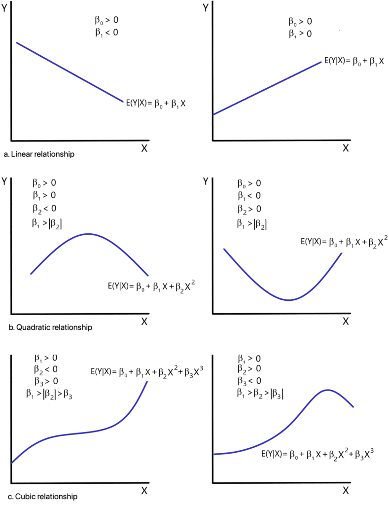
Figure 8.1 contains graphs of linear, quadratic and cubic polynomial relationships. A linear relationship has constant slope (either positive or negative). Quadratic relationships are either U-shaped or have a shape that resembles an inverted-U. A cubic relationship appears to be shaped roughly like either the letter “S ” or an inverted “S.” It may be observed that the number of turning points (the number of times that the function changes direction) for a polynomial is, at most, equal to [latex]k-1[/latex].

8.2.1 Example: Cubic cost function

In virtually any introductory microeconomics text, the short-run cost curve is generally drawn in a manner resembling the curve appearing in the lower left-hand corner of Figure 8.1. This suggests that a short-run cost function may be specified as:

\begin{equation}C_{t}=\beta _{0}+\beta _{1}Q_{t}+\beta _{2}Q_{t}^{2}+\beta_{3}Q_{t}^{3}+u_{t} \tag{8.10}\end{equation}

where:

• C[latex]_{t}[/latex]= total cost at time [latex]t[/latex]
• Q[latex]_{t}[/latex] = quantity of output produced at time [latex]t[/latex]

To estimate the parameters of this model, an econometrician can use the transformations:

\begin{equation*}
X_{1t}=Q_{t}
\end{equation*}
\begin{equation*}
X_{2t}=Q_{t}^{2}
\end{equation*}
\begin{equation*}
X_{3t}=Q_{t}^{3}
\end{equation*}

Thus, equation 8.10 may be restated as:

\begin{equation}
C_{t}=\beta _{0}+\beta _{1}X_{1t}+\beta _{2}X_{2t}+\beta _{3}X_{3t}+u_{t} \tag{8.11}
\end{equation}

The parameters of equation 8.11 may be estimated by OLS estimation techniques (assuming that all of the other conditions of the classical regression model are satisfied).

8.3 The reciprocal transformation

Suppose that the relationship between two variables is captured by the equation:

\begin{equation} \tag{8.12}
Y_i=\beta_0+\beta _1\frac 1{X_i}+u_i
\end{equation}

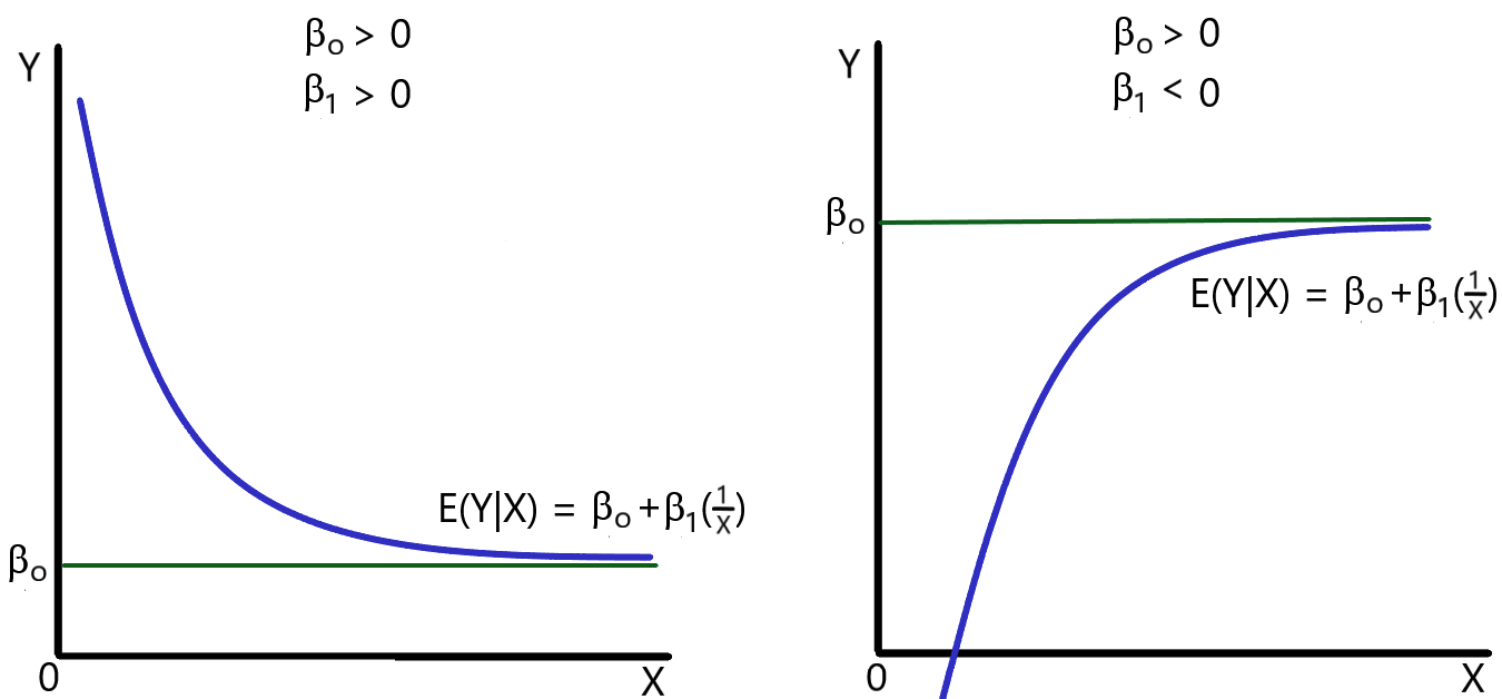
An examination of equation 8.12 indicates that in this model:

• [latex]Y[/latex] tends to decrease when [latex]X[/latex] increases if [latex]\beta_1[/latex] is positive (since [latex]1/X[/latex] declines as [latex]X[/latex] increases);
• [latex]Y[/latex] tends to increase when [latex]X[/latex] increases if [latex]\beta_1[/latex] is negative;
• [latex]E(Y|X)[/latex] asymptotically approaches the value [latex]\beta_o[/latex] as [latex]X[/latex] tends toward infinity.
• When [latex]\beta_1[/latex] is positive, [latex]E(Y|X)[/latex] approaches positive infinity as [latex]X[/latex] tends toward zero (since [latex]1/X_i[/latex] tends toward infinity as [latex]X[/latex] tends toward zero). [latex]E(Y|X)[/latex] approaches negative infinity as [latex]X[/latex] tends toward zero when [latex]\beta_1[/latex] is negative.

Figure 8.2  illustrates two possible forms of this function. Notice that the curve is downward sloping when [latex]\beta_{1}[/latex] is positive and is upward sloping when [latex]\beta_{1}[/latex] is negative. In both cases, the parameter [latex]\beta _{0}[/latex]is positive. If [latex]\beta _{0}[/latex] were negative, the graph would be similar, but the function would asymptotically approach a negative value (= [latex]\beta_{0}[/latex]).

Using the technique discussed above, this model can be transformed into a linear specification by defining a new variable, [latex]Z_{i}[/latex], as:

\begin{equation*}
Z_{i}=\frac{1}{X_{i}}
\end{equation*}

When this definition is substituted into equation 8.12, the transformed equation is:

\begin{equation}
Y_{i}=\beta _{0}+\beta _{1}Z_{i}+u_{i} \tag{8.13} \end{equation}

Since equation 8.13 is linear in variables, the parameters [latex]\beta_{0}[/latex] and [latex]\beta _{1}[/latex] can be estimated using an OLS procedure. In interpreting the results, however, be sure to observe that a positive value for [latex]\beta_{1}[/latex] indicates that [latex]Y[/latex] and [latex]X[/latex] are inversely related.

The reciprocal transformation is often used for models in which:

• a one-unit change in the independent variable results in progressively smaller changes in the level of the dependent variable;
• the dependent variable asymptotically approaches a finite value ([latex]\beta_o[/latex]) as an independent variable tends toward infinity; and
• the dependent variable tends toward positive or negative infinity as the independent variable tends toward zero.

8.3.1 Example: The Phillips curve

The Phillips curve provides a natural application for the reciprocal transformation. In its original form, the Phillips curve was specified as a relationship between the rate of change in money wages and the unemployment rate. Later studies focused on the relationship between the inflation rate and the unemployment rate. These early studies found a relationship between the inflation rate (or the rate of change in money wages) and the unemployment rate that resembled the graph appearing on the left-hand side of Figure 8.2 (although [latex]\beta_{o}[/latex] was generally found to be negative in these studies).

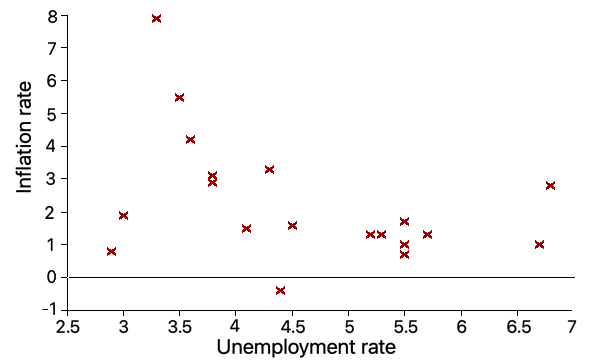
Figure 8.3 contains a scatterplot of the relationship between the inflation rate and the civilian unemployment rate in the U.S. during the period 1950 to 1969.^[2] This scatterplot suggests that a reciprocal relationship between the inflation rate and the unemployment rate is an appropriate specification. Thus, a simple Phillips curve may be estimated of the form:
\begin{equation}
\text{Inflation rate}_{t}\text{ = }\beta _{0}+\beta _{1}\left( \frac{1}{\text{Unemployment rate}_{t}}\right) +u_{t} \tag{8.14} \end{equation}
When the parameters of equation 8.14 are estimated using OLS, the estimated equation is:
\begin{equation}
\widehat{\text{Inflation\ rate}}_{t}\text{= }\underset{(-0.69)}{-1.12}+\underset{(2.11)}{14.52}\left( \frac{1}{\text{Unemployment rate}_{t}}\right) \tag{8.15}
\end{equation}
\begin{equation*}
\text{(}t\text{-ratios in parentheses)}
\end{equation*}
While the intercept term is insignificant at all conventional levels, the estimated coefficient [latex]\hat{\beta}_{1}[/latex] is significantly greater than zero at a 5% significance level. As noted above, a positive coefficient multiplying the reciprocal of the unemployment rate implies an inverse relationship between the unemployment and inflation rates. Thus, this result suggests that the Phillips curve (in this time period) was downward sloping. As the unemployment rate rose, the inflation rate tended to decline.

8.4. Log transformations

8.4.1 Log-Log models

Suppose that the relationship between a dependent variable ([latex]Y[/latex]) and a set of independent variables ([latex]X_1,X_2,\ldots X_k[/latex]) is given by: \begin{equation*}
Y_i=\beta_0X_{1i}^{\beta _1}X_{2i}^{\beta _2}\cdots X_{ki}^{\beta _k}e^{u_i} \end{equation*}
where:

• [latex]u_i[/latex] is a random error term}
• [latex]e[/latex] = base of natural logarithm

This type of exponential function may be converted into a linear form by taking the natural log of both sides of the equation. This results in:

\begin{equation} \tag{8.16}
\ln (Y_i)=\ln (\beta_0)+\beta _1\ln (X_{1i})+\beta _2\ln (X_{2i})+\ldots +\beta _k\ln (X_{ki})+u_i
\end{equation}
Using the transformations:
\begin{equation*}
\tilde Y_i=\ln (Y_i)
\end{equation*}
\begin{equation*}
\tilde \beta _o=\ln (\beta _o)
\end{equation*}
\begin{equation*}
\tilde X_{1i}=\ln (X_{1i})
\end{equation*}
\begin{equation*}
\tilde X_{2i}=\ln (X_{2i})
\end{equation*}
\begin{equation*}
\vdots
\end{equation*}
\begin{equation*}
\tilde X_{ki}=\ln (X_{ki})
\end{equation*}
equation 8.16 can be restated as:
\begin{equation} \tag{8.17}
\tilde Y_i=\tilde \beta_0+\beta _1\tilde X_{2i}+\beta _1\tilde X_{2i}+\ldots +\beta _k\tilde X_{ki}+u_i
\end{equation}
The parameters of equation 8.17 can be estimated using the OLS method (as long as all of the other assumptions of the classical regression model are satisfied).
Since both the dependent and independent variables are expressed in log form, this type of model specification is referred to as a double-log (or log-log) mode}. One interesting feature of models of this sort is that each of the slope parameters [latex]\beta_{1},\beta_{2},\ldots,\beta_{k}[/latex]^[3] provides a measure of the percentage change in the dependent variable that occurs when there is a one-percent change in the corresponding independent variable (holding all other variables constant). In other words:^[4]}
\begin{equation*}
\beta _{j}=\frac{\% \Delta \text{ in }Y}{\% \Delta \text{ in }X_{j}} \end{equation*}
In economic terms, each of the estimated slope coefficients in the transformed model serves as a measure of the elasticity of [latex]Y[/latex] with respect to [latex]X[/latex]. This is a property that is often exploited by econometricians who wish to estimate elasticities. This topic is discussed in more detail below.

A double-log model is appropriate when:

• the dependent and independent variables are always greater than zero, and
• it is anticipated that a one-percent change in an independent variable always results in a constant percentage change in the dependent variable.

Let’s examine some common applications of the double-log specification.

8.4.2 Example: Demand elasticities

In introductory economics courses, demand and supply curves are generally represented as linear relationships. There is no reason, however, to assume that these demand and supply curves are necessarily linear. In a variety of empirical studies, a double-log specification has been found to represent demand relationships as well as, or better than, a linear specification.
Consider the following demand curve for good [latex]X[/latex]:
\begin{equation}
Q_d=\beta_0P_X^{\beta _1}P_Y^{\beta _2}P_Z^{\beta _3}I^{\beta _4} \tag{8.18}
\end{equation}
where:

• [latex]Q_d[/latex] = quantity of good [latex]X[/latex] demanded}
• [latex]P_X[/latex] = price of good [latex]X[/latex]
• [latex]P_Y[/latex] = price of good [latex]Y[/latex]
• [latex]P_Z[/latex] = price of good [latex]Z[/latex]
• [latex]I[/latex] = consumer income

This demand equation may be converted into a linear form by taking the natural log of both sides of equation 8.18 The resulting equation is:
\begin{equation*}
\ln (Q_d)=\ln (\beta_0)+\beta_1\ln (P_X)+\beta _2\ln (P_Y)+\beta_3\ln (P_Z)+\beta_4\ln (I)
\end{equation*}

This equation provides a linear relationship between the log of quantity demanded and the logs of the price and income variables. Since it is likely that observed data will not exactly fit this equation, a random error term can be added to capture the observed demand relationship at time [latex]t[/latex]:

\begin{equation}
\ln (Q_{dt})=\ln (\beta_0)+\beta _1\ln (P_{Xt})+\beta _2\ln (P_{Yt})+\beta _3\ln (P_{Zt})+\beta _4\ln (I_t)+u_t \tag{8.19}
\end{equation}

The parameters of equation 8.19 can be estimated by OLS techniques using the procedure discussed above (assuming that all of the other assumptions of the classical regression model are satisfied).

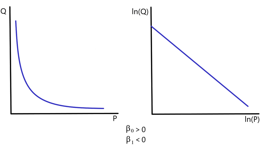
Figure 8.4 illustrates the relationship that exists between the price of the good and the quantity demanded (holding income and the prices of other goods constant) under a double-log specification. Notice that the graph of the relationship between the log of quantity demanded and the log of price is linear under this specification. (It should be noted that the coefficient [latex]\beta_{1}[/latex] is negative in this example.)

As noted above, under the double-log specification, each of the coefficients [latex]\beta_{1},\beta_{2},\ldots,\beta_{k}[/latex] provides a measure of the percentage change in the dependent variable that occurs when there is a one-percent change in the corresponding independent variable, holding all of the other independent variables constant. In other words:

\begin{equation*}
\beta _{1}=\frac{\%\Delta \text{ in }Q_{d}}{\%\Delta \text{ in }P_{X}} \end{equation*}
\begin{equation*}
\beta _{2}=\frac{\%\Delta \text{ in }Q_{d}}{\%\Delta \text{ in }P_{Y}} \end{equation*}
\begin{equation*}
\beta _{3}=\frac{\%\Delta \text{ in }Q_{d}}{\%\Delta \text{ in }P_{Z}} \end{equation*}
\begin{equation*}
\beta _{4}=\frac{\%\Delta \text{ in }Q_{d}}{\%\Delta \text{ in }I} \end{equation*}

Thus, each of these parameters equals an elasticity. In this model, the coefficient [latex]\beta_{1}[/latex] equals the price elasticity of demand. This is a measure of the sensitivity of quantity demanded to a change in the price of the good. The coefficient [latex]\beta_{2}[/latex] equals the cross-price elasticity of demand between goods [latex]X[/latex] and [latex]Y[/latex]. A positive value of [latex]\beta_{2}[/latex] indicates that goods [latex]X[/latex] and [latex]Y[/latex] are substitutes; a negative value indicates that [latex]X[/latex] and [latex]Y[/latex] are complements. In a similar manner, the coefficient [latex]\beta_{3}[/latex] equals the cross-price elasticity of demand between goods [latex]X[/latex] and [latex]Z[/latex]. The parameter [latex]\beta_{4}[/latex] is the income elasticity of demand for good [latex]X[/latex]. A positive value for [latex]\beta_{4}[/latex] indicates that good [latex]X[/latex] is a normal good; [latex]\beta_{4}[/latex] is negative if good [latex]X[/latex] is an inferior good.

Many economics textbooks contain lists of estimated price elasticities of demand, cross-price elasticities of demand, and income elasticities of demand. The estimates are typically derived using a procedure equivalent to that discussed above.

It should be noted, however, that one cannot always use observed data on prices and quantities to estimate the parameters of a demand equation. In a competitive market, the equilibrium price and quantity at a point in time is determined by the interaction of market demand and supply. Suppose that data is collected on the equilibrium prices and quantities of a good sold in a competitive market. Would the observed relationship represent a demand curve or a supply curve? In fact, this observed relationship will generally represent neither a demand curve nor a supply curve. To estimate a demand relationship in these circumstances, it is necessary to estimate the parameters of both the demand and supply equations simultaneously.

Estimation procedures for simultaneous equation models of this sort are discussed in Chapter 15.

A demand equation, however, may be estimated using OLS techniques if the data on quantity demanded was gathered directly from a survey of consumers.

Surveys of this sort may be conducted by:

• market research firms interested in estimating demand elasticities, or
• large corporations attempting to estimate the demand for their product.

8.4.3 Example: Cobb-Douglas production function

The Cobb-Douglas production function provides another interesting application of the double-log specification. Suppose that there are only two inputs used to produce output: labor ($L$) and capital ($K$). A production function captures the relationship that exists between the level of input usage and the maximum amount of output that can be produced (assuming efficient production). The general form of a production function is:

\begin{equation*}Q=f(L,K)\end{equation*}

In the particular case of a Cobb-Douglas production function, this becomes:^[5]

\begin{equation}
Q=\beta _{0}L^{\beta _{1}}K^{\beta _{2}} \tag{8.20} \end{equation}
The Cobb-Douglas production function can be converted into a linear form by taking the natural log of both sides of equation 8.20. The resulting equation is:
\begin{equation*}
\ln (Q)=\ln (\beta _{0})+\beta _{1}\ln (L)+\beta _{2}\ln (K) \end{equation*}
Allowing for random errors, the observed relationship between inputs and output becomes:
\begin{equation}
\ln (Q_{i})=\ln (\beta _{0})+\beta _{1}\ln (L_{i})+\beta _{2}\ln (K_{i})+u_{i} \tag{8.21}
\end{equation}
Since this is a double-log specification, the coefficients [latex]\beta_1[/latex] and [latex]\beta_2[/latex] can be interpreted as the percentage change in output resulting from a one-percent increase in the level of labor or capital, respectively.
In mathematical terms, this can be expressed as:
\begin{equation*}
\beta _1=\frac{\%\Delta \text{ in }Q}{\%\Delta \text{ in }L} \end{equation*}
and
\begin{equation*}
\beta _2=\frac{\%\Delta \text{ in }Q}{\%\Delta \text{ in }K} \end{equation*}
Equation 8.21 can be transformed into a linear form by defining:
\begin{equation*}
Y_i=\ln (Q_i)
\end{equation*}
\begin{equation*}
\beta _0^{\prime }=\ln (\beta _0)
\end{equation*}
\begin{equation*}
X_{1i}=\ln (L_i)
\end{equation*}
\begin{equation*}
X_{2i}=\ln (K_i)
\end{equation*}
Thus, equation 8.21 can be restated as:
\begin{equation}
Y_i=\beta _0^{\prime }+\beta _1X_{1i}+\beta _2X_{2i}+u_i\tag{8.22}
\end{equation}
An OLS estimation procedure may be used to estimate the parameters of equation 8.22. The estimated coefficients [latex]\hat{\beta}_{1}[/latex] and [latex]\hat{\beta}_{2}[/latex] serve as estimates of the parameters [latex]\beta _{1}[/latex] and [latex]\beta_{2}[/latex] that appear in the production function (equation 8.20). The estimated coefficient [latex]\hat{\beta}_{0}^{\prime }[/latex], however, serves as an estimator of [latex]\ln (\beta _{o})[/latex]. In mathematical terms:
\begin{equation*}
\hat{\beta}_{0}^{\prime }=\widehat{\ln (\beta_{o})}
\end{equation*}
This can be converted into an estimate of [latex]\beta_{0}[/latex] by noting that:

\begin{equation*}
\beta_{0}=e^{\ln (\beta _{0})}
\end{equation*}
Thus, the estimated value of  [latex]\beta _{0}[/latex] is:^[6]
\begin{equation}
\hat{\beta}_{0}=e\widehat{^{\ln (\beta _{o})}} \tag{8.23} \end{equation}
or
\begin{equation*}
\hat{\beta}_{0}=e^{\hat{\beta}_{0}^{\prime }}
\end{equation*}
One of the interesting features of a Cobb-Douglas production function is that it exhibits:^[7]}

• constant returns to scale if [latex]\beta_1+\beta _2=1,[/latex]
• increasing returns to scale if [latex]\beta_1+\beta_2>1[/latex], or
• decreasing returns to scale if [latex]\beta _{1}+\beta _{2}<1[/latex].

Suppose that an econometrician wishes to examine whether a particular production function exhibits increasing returns to scale. If it is assumed that the production function is a Cobb-Douglas production function, then OLS estimation techniques can be used to estimate the parameters of the function (following the procedure discussed above). If the econometrician wishes to determine whether the production process exhibits constant returns to scale, the appropriate hypotheses are:

\begin{equation*}
\text{H}_{0}\text{: }\beta _{1}+\beta _{2}=1
\end{equation*}
and
\begin{equation*}
\text{H}_{1}\text{: }\beta _{1}+\beta _{2}\neq 1
\end{equation*}
If the null hypothesis can be rejected at the selected significance level, then the econometrician can reject the null hypothesis of constant returns to scale. A procedure for conducting hypothesis tests of this sort was discussed in Chapter 7.

8.4.4 Semi-log models

As noted above, a double-log model is used if it is believed that a one-percent change in the independent variable(s) results in a constant percentage change in the level of the dependent variable. Under some circumstances, however, it is likely that a one-unit change in an independent variable results in a constant percentage change in the dependent variable. It is also possible that a one-percent change in an independent variable results in a constant change in the level of the dependent variable. Let’s consider two functional forms that allow for relationships such as these.

Consider the functions:
\begin{equation}
Y=\beta_{0}+\beta_{1}\ln (X_{1})+\beta _{2}\ln (X_{2})+\ldots +\beta _{k}\ln (X_{k}) \tag{8.24}
\end{equation}
and
\begin{equation}
\ln (Y)=\beta_{0}+\beta_{1}X_{1}+\beta _{2}X_{2}+\ldots +\beta _{k}X_{k} \tag{8.25}
\end{equation}

Econometric models of this sort are referred to as semi-log models since the log term(s) appear on only one side of the equation.

Specifications such as those in equation 8.24 are sometimes called linear-log models since the log variables appear only on the right-hand side of the equation. In a log-linear model,^[8] the log variable appears only on the left-hand side of the equation (as in equation 8.25). In a linear-log model, a one-percent change in an independent variable results in a given change in the level of the dependent variable. Under a log-linear model, however, a one-unit change in an independent variable results in a constant percentage change in the dependent variable.^[9] Let’s examine these two specifications in more detail.

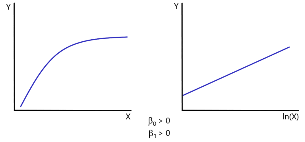
8.4.5 Linear-log model

Model specifications such as those in equation 8.24 are used when it is anticipated that the percentage change in an independent variable has a constant effect on the level of the dependent variable. In this case, a given change in the level of an independent variable will result in progressively smaller changes in the level of the dependent variable. A bivariate form of this function is depicted in Figure 8.5.

One possible application of this model is found in the estimation of short-run production functions. In the short run, the law of diminishing returns indicates that the introduction of additional units of a variable input (in a production process in which some inputs are fixed) will result in progressively smaller increases in output. A linear-log function may capture this relationship quite effectively. It should be noted, however, that under a linear-log model, the slope of the function remains positive (although it approaches zero as [latex]X_i[/latex] increases). Thus, this particular function would be appropriate only for production processes in which the marginal product of the variable input approaches, but never equals, zero.

Consider the relationship that exists between expenditures on pollution abatement and the reduction in the quantity of pollution. Suppose society were to increase the level of spending devoted to pollution abatement. Some types of pollution can be reduced at relatively little cost to society; others require more costly remedies. The first pollution abatement programs implemented would be expected to involve relatively large reductions in pollution per dollar of expenditure (if the program is efficiently administered). As the level of spending increases, it would be expected that each additional dollar of spending would result in progressively smaller reductions in the amount of pollution. The relationship between spending on pollution abatement and the level of pollution might be expected to resemble that depicted in Figure 8.5. An econometrician estimating a relationship between the level of pollution and spending on pollution abatement might consider a model of the form:^[10]}
\begin{equation*}
\text{Pollution abatement}_{t}=\beta _{0}+\beta _{1}\ln (\text{spending on pollution abatement}_{t})+u_{t}
\end{equation*}
Obviously, a more complete specification would include other independent variables as well. It would be reasonable, however, to use the log of spending on pollution abatement as one of these independent variables.

Under a linear-log specification, each of the slope coefficients can be expressed as:^[11]
\begin{equation*}
\beta _{j}=\frac{\Delta Y}{\Delta X_{j}/X_{j}}
\end{equation*}
or
\begin{equation*}
\beta _{j}=\frac{\Delta Y}{\left( \%\Delta \ \text{in}\ X_{j}\right) /\text{ }100\%}
\end{equation*}
Thus, each coefficient provides a measure of the change in the level of the dependent variable that occurs when there is a 100% increase in the corresponding independent variable.

8.4.6 Log-linear model

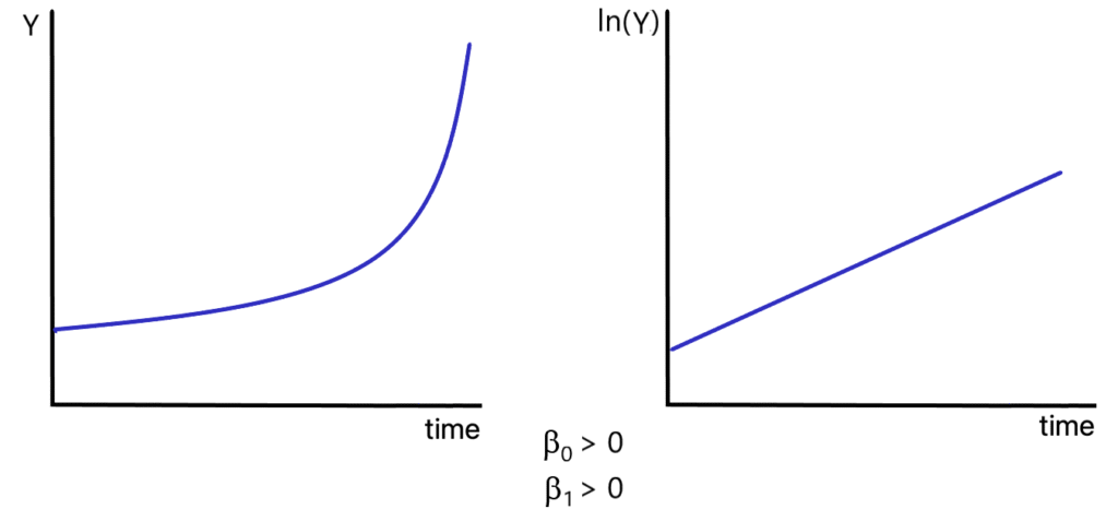
Log-linear models (as in equation 8.25) are used when it is anticipated that a one-unit change in an independent variable will result in a constant percentage change in the dependent variable. One of the most common applications of this model involves estimating the time path of an economic time series that grows at a constant rate. The general formula for such a relationship is given by:

\begin{equation}
Y_{t}=Ae^{rt} \tag{8.26}
\end{equation}
where:

• Y[latex]_{t}[/latex] = value of variable at time [latex]t[/latex]
• [latex]A[/latex] = initial value of [latex]Y_{t}[/latex] at [latex]t=0[/latex]
• [latex]e[/latex] = base of natural logarithm
• [latex]r[/latex] = instantaneous rate of growth

(A mathematically sophisticated reader will note that equation 8.26 is also the formula used to determine the value at time [latex]t[/latex] of a financial asset that receives interest at a rate of [latex]r[/latex] under continuous compounding.) This formula may be converted into a linear form by taking the logs of both sides of equation 8.26:^[12]

\begin{equation}
\ln (Y_{t})=\ln (A)+rt \tag{8.27}
\end{equation}

Figure 8.6 contains graphs of the time path of [latex]Y_{t}[/latex] and [latex]\ln(Y_{t})[/latex].

Adding a random error term, equation 8.27 may be rewritten as:

\begin{equation}
\ln(Y_t)=\beta_0+\beta_1t+u_t \tag{8.28}
\end{equation}
where the parameters [latex]\beta_0[/latex] and [latex]\beta_1[/latex] are defined as:

\begin{equation*}
\beta _0=\ln (A)
\end{equation*}
and
\begin{equation*}
\beta_1=r
\end{equation*}
Equation 8.28 is now written in a form that is amenable to OLS estimation. The dependent variable is the log of the time-series variable, the independent variable equals the time at which each value of the dependent variable is observed. The estimated value of [latex]\beta_1[/latex] serves as a direct measure of the instantaneous rate of growth of the variable [latex]Y_t[/latex]. An example of this procedure is considered below.

The estimation of earnings equations provides another common example of a log-linear model. Earnings equations are generally specified as:

\begin{equation}
\ln (\text{earnings}_{i})=\beta _{0}+\beta _{1}X_{1i}+\beta _{2}X_{2i}+\ldots +\beta _{k}X_{ki}+u_{i} \tag{8.29}
\end{equation}

where the variables [latex]X_{1i},\ldots, X_{ki}[/latex] include measures of ability, work experience and any demographic characteristics that may affect an individual’s earnings. A primary reason for this specification is that when individuals receive wage or salary increases, the increases are generally specified as a [latex]percentage increase[/latex] over the previous wage or salary. Thus, an additional year of work experience will result in a fixed percentage increase in earnings, not a fixed dollar increase. Thus, it is reasonable to assume that the log of earnings is a function of the level of work experience.

Under the log-linear specification, each of the coefficients [latex]\beta_{1},\beta_{2},\ldots ,\beta_{k}[/latex] equals:^[13]
\begin{equation*}
\beta _{j}=\frac{\Delta Y/Y}{\Delta X_{j}}
\end{equation*}
or
\begin{equation*}
\beta _{j}=\frac{\left( \%\Delta \ \text{in}\ Y\right) /\text{ }100\%}{\Delta \ X_{j}}
\end{equation*}
Alternatively:
\begin{equation*}
\beta _{i}\times 100\%=\%\Delta \text{ in }Y\text{ that results from a one-unit change in }X_{i}
\end{equation*}
Thus, when an econometrician estimates an earnings equation (such as the one appearing in equation 8.29, the estimated coefficients [latex]\beta_{1},\ldots,\beta_{k}[/latex] can be used, for example, to estimate the percentage change in earnings that results from:

• a one-year increase in educational attainment,
• a one-month increase in work experience, or
• the presence of a particular demographic characteristic (such as race, marital status, or gender).

8.4.7 Example: U.S. per capita health care expenditures

The recent interest in national health insurance is provoked, in large part, by the rapid increase in health care expenditures in the U.S. Figure 8.7 contains a graph of per capita health care expenditures from 1960 to 1998.^[14] This graph indicates that per capita health care expenditures appear to be growing in a manner consistent with the log-linear model discussed above.

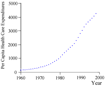
To determine the instantaneous rate of growth of per capita health care expenditures, a model can be specified as:
\begin{equation*}
\ln (\text{Health}_{t})=\beta_{0}+\beta_{1}\text{Year}_{t}\text{ }+u_{t} \end{equation*}

where: Health[latex]_{t}[/latex] = per capita health care expenditures in year [latex]t[/latex]

When the parameters of this equation are estimated through OLS, the estimated equation is:
\begin{equation}
\widehat{\ln (\text{Health}_{t})}=\underset{(-64.28)}{-185.69}+\underset{% (66.71)}{0.097}\text{Year}_{t} \tag{8.30}
\end{equation}
\begin{equation*}
\overline{\text{R}}^{2}=0.99
\end{equation*}
\begin{equation*}
\text{(}t\text{-ratios in parentheses)}
\end{equation*}
Thus, this estimated equation indicates that health care expenditures are growing at a rate of 9.7% per year (the compound rate of growth will be higher). This rate of increase is substantially greater than the inflation rate during this period.

8.4.8 Caution: log transformations and observations equal to zero

Virtually all novice econometricians at some point attempt to execute a log transformation using a regression package and receive an error message from the computer that resembles one of the following:

• givision by zero error,
• floating point exception,
• divide overflow,
• illegal operand,
• illegal operation, or
• some other, occasionally more informative, response.

This error is nearly always caused by an attempt to take the log of an observation which is less than or equal to zero. Since [latex]\ln (x)[/latex] approaches negative infinity as [latex]x[/latex] tends toward zero, the log of zero is undefined (as is the log of negative numbers). Before attempting to apply the log transformation to a dependent or independent variable, it is important to check to be sure that the variable is always greater than zero. When dealing with data on individual income, for example, it is not uncommon to find some individuals reporting a value of zero for some categories of income.
What can be done if one or more observations contain a value equal to zero?
Three solutions are commonly used:

• Select only those observations that contain positive values of the affected variable and perform the log transformation and regression procedure using only these observations. This procedure, however, introduces the possibility of sample selection bias (since a nonrandom sample is being used to generate estimates). Fortunately, several techniques exist that make it possible to generate consistent estimates in sample selectivity models. Several of these procedures are discussed in Chapter 14.
• Apply an alternative model specification. This might, for example, involve replacing a double-log or semi-log model with a polynomial model.^[15]}
• In cases in which a nonnegative variable sometimes takes on a value of zero, some authors suggest replacing each value of zero with a small quantity (such as 0.00001). This would allow the log transformation to be applied. Many econometricians, however, argue that it is better to select a model that appropriately represents the data-generating process rather than trying to “adjust” the data to fit the model.