Chapter 9 – Functional Form II: Further Topics
In the previous chapter, it was shown that many nonlinear models may be converted into a linear form by an appropriate redefinition of variables. Transformations of this sort substantially expand the range of models that may be estimated using OLS techniques. In this chapter, a number of additional topics related to the choice of functional form will be examined. These topics include:
- the effect of changing the units in which variables are measured;
- the introduction of “interaction terms” that capture the joint effect of two variables; and
- allowing for qualitative independent variables.
9.1 Units of measurement
Variables may be measured in terms of many different units. In estimating aggregate macroeconomic models, data may be measured in terms of “dollars,” “thousands of dollars,” or “millions of dollars.” Prices may be expressed in terms of dollars from different base years. Distances may be measured in inches, feet, yards, miles, meters, or kilometers. The quantity of oil consumed may be measured in terms of gallons, liters, or thousand gallons (or liters). One obvious question is: What impact will the choice of units of measurement have upon the magnitude of regression coefficients?
To discuss this issue, we can note that changing the units in which a variable is measured involves a linear transformation of the affected variable. Thus, if the original variable is [latex]X[/latex], the transformed variable can be written as:
[latex]\tilde X=cX[/latex]
where [latex]c[/latex] is a positive constant. If the original variable ([latex]X[/latex]) is measured in terms of dollars, and an econometrician wishes to convert it to a variable ([latex]\tilde X[/latex]) measured in terms of thousands of dollars, the constant [latex]c[/latex] would equal 1/1000.
Let’s examine a bivariate relationship of the form:
[latex]Y_{i}=\beta _{o}+\beta _{1}X_{i}+u_{i} \tag{9.1}[/latex]
Suppose that an econometrician chooses to measure the dependent and independent variables in different units of measurement. The transformed dependent and independent variables are defined as:[1]
[latex]\tilde{Y}_{i}=c_{1}Y_{i} \tag{9.2}[/latex]
and
[latex]\tilde{X}_{i}=c_{2}X_{i} \tag{9.3}[/latex]
Thus, using the definitions in equations 9.2 and 9.3, equation 9.1 may be expressed in terms of the transformed variables as:
[latex]\frac{1}{c_{1}}\tilde{Y}_{i}=\beta_{0}+( \frac{1}{c_{2}}) \beta_{1}\tilde{X}_{i}+u_{i}[/latex]
Multiplying by sides of this equation by [latex]c_{1}[/latex], this becomes:
[latex]\tilde{Y}_{i}=c_{1}\beta_{0}+( \frac{c_{1}}{c_{2}}) \beta_{1}\tilde{X}_{i}+c_{1}u_{i} \tag{9.4}[/latex]
Equation 9.4 may be restated as:
[latex]\tilde{Y}_{i}=\beta _{o}^{\prime }+\beta _{1}^{\prime }\tilde{X} _{i}+u_{i}^{\prime } \tag{9.5}[/latex]
where:
[latex]\beta_{0}^{\prime }=c_{1}\beta_{0} \tag{9.7}[/latex]
[latex]\beta _{1}^{\prime }=\left( \frac{c_{1}}{c_{2}}\right) \beta_{1}[/latex]
and
[latex]u_{i}^{\prime }=c_{1}u_{i}[/latex]
When an econometrician estimates the parameters of the transformed model in equation 9.5, the relationship between the estimated and the original parameters is given by the definitions in 9.6. The relationships between the estimated parameters in the original and transformed equations are given by:[2]
[latex]\hat{\beta}_{0}^{\prime }=c_{1}\hat{\beta}_{0} \tag{9.7}[/latex]
and:
[latex]\hat{\beta}_{1}^{\prime }=( \frac{c_{1}}{c_{2}}) \hat{\beta}_{1} \tag{9.8}[/latex]
Equations 9.7 and 9.8 indicate that changing the scale of the dependent and/or independent variables results in a well-defined effect on the magnitude of the slope and intercept coefficients. If the dependent variable is redefined so that it is larger in magnitude, the slope and intercept coefficients will increase by the same proportion. A redefinition that reduces the magnitude of only the dependent variable results in a proportionate reduction in the scale of the intercept and slope coefficients.
Suppose, for example, that a dependent variable initially measured in terms of thousands of dollars is converted into a dependent variable that is measured in dollars (the new dependent variable equals 1,000 [latex]\times[/latex] original variable). When the dependent variable is measured in dollars, the slope and intercept terms will be 1,000 times larger than the corresponding estimates when the dependent variable is measured in terms of thousands of dollars.
If, however, an independent variable originally measured in terms of thousands of dollars is transformed into an independent variable measured in term of dollars, then the estimated slope coefficient will be 1/1,000 of its value in the original model. The intercept coefficient will remain the same. In general, a change in the scale of any single independent variable will affect only the magnitude of the corresponding slope coefficient.
In many cases (particularly those involving aggregate relationships), an econometrician will rescale both the dependent and independent variable by the same amount. For example, all terms in a consumption function might be expressed in terms of millions of dollars. In this case, the scale coefficients [latex]c_{1}[/latex] and [latex]c_{2}[/latex] are equal. An inspection of equations 9.7 and 9.8 indicates that a rescaling of this sort will affect only the intercept. The slope coefficient(s) will remain the same under these conditions.
9.1.1 Hypothesis tests and changes in the units of measurements
While changes in the units of measurements will affect the magnitude of intercept and slope coefficients, the [latex]t[/latex] ratios used to test the significance of these parameters will be unaffected.
Proof:
As noted in Chapter 3, if the variable [latex]X[/latex] has a variance of [latex]\sigma ^2[/latex], then the transformed variable [latex]cX[/latex], has a variance equal to:
[latex]\text{var}(cX)=c^2\text{var}(X)[/latex]
Thus, when the parameters of the transformed equation (equation 9.5) are estimated, the variances of the estimated intercept and slope parameters are:
[latex]\text{var}(\beta_0^{\prime })=c_1^2\text{var(}\beta_0\text{)} \tag{9.9}[/latex]
and
[latex]\text{var}(\beta_1^{\prime })=( \frac{c_1}{c_2}) ^2\text{var}( \beta_1)[/latex]
If an econometrician wished to test to determine whether the intercept or slope parameters are significantly different than zero, the appropriate [latex]t[/latex] ratios are:
[latex]t_{\hat{\beta}_0^{\prime }}=\frac{\hat{\beta}_o^{\prime }}{\sqrt{var(\beta_0^{\prime })}}[/latex]
and
[latex]t_{\hat{\beta}_1^{\prime }}=\frac{\hat{\beta}_1^{\prime }}{\sqrt{var(\beta_1^{\prime })}}[/latex]
Using the definitions in 9.7 9.8, and 9.9, these [latex]t[/latex] ratios may be restated as:
[latex]t_{\hat{\beta}_0^{\prime}} = \frac{c_1 \hat{\beta}_0}{\sqrt{c_1^2 \text{var}(\beta_0)}} = \frac{\hat{\beta}_0}{\sqrt{\text{var}(\beta_0)}}[/latex]
and
[latex]t_{\hat{\beta}_1^{\prime }}=\frac{\left( \frac{c_1}{c_2}\right) \hat{\beta}_1 }{\sqrt{( \frac{c_1}{c_2}) ^2\text{var}(\beta _1)}}=\frac{\hat{ \beta}_1}{\sqrt{\text{var}(\beta_1)}}[/latex]
As these equations indicate, the estimated [latex]t[/latex] ratios in the transformed model are exactly the same as the [latex]t[/latex] ratios in the original specification. Thus, hypothesis tests involving these coefficients are not affected by the choice of units of measurement.
9.1.2 Caution: significant digits
Most economic variables are reported to only three to five significant digits. For example, annual U.S. consumption and income data is generally reported in terms of billions of dollars. In 2025, real consumption expenditures are reported as $23,852.994 billion (in chained 2017 dollars).[3]}It is unlikely, however, that the level of real consumption spending was exactly equal to $23,852.994,000,000. Instead, consumption and income estimates are accurate (at best) to hundreds of millions of dollars.
Most regression packages will report 8 or more digits when listing estimated regression coefficients. It is unreasonable, however, to report intercept and slope coefficients that are more accurate than the data from which they are estimated. A simple rule of thumb is to report regression results using a number of significant digits that is consistent with that used in recording the data.
9.2 Interaction effects
In many economic models, changes in the level of one variable affects the magnitude of the impact resulting from a one-unit change in another variable. For example, in many production processes, an increase in the level of capital will increase the marginal product of labor (the additional output that is produced when there is a one-unit increase in the level of labor use). It is also quite possible that individuals who are more able (as measured by IQ or SAT scores) may gain more from an additional year of work experience than those individuals who are less able.
Fortunately, there is a convenient method that makes it possible to capture interaction effects of this sort. Suppose that each of the independent variables [latex]X[/latex] and [latex]Z[/latex] affects a dependent variable, [latex]Y[/latex], both directly and indirectly through its interaction with the other independent variable. A model may be specified of the form:
[latex]Y=\beta _o+\beta _1X+\beta _2Z+\beta _3(XZ) \tag{9.10}[/latex]
The model specified in equation 9.10 differs from earlier regression models in that it includes an interaction term that equals the product of two independent variables.
Let’s examine the effect of a change in the level of [latex]X[/latex] on the dependent variable (holding the level of [latex]Z[/latex] constant). To see this, it will be convenient to restate equation 9.10 as:
[latex]Y=\beta_0+(\beta _1+\beta _3Z)X+\beta _2Z \tag{9.11}[/latex]
Suppose that the level of [latex]X[/latex] changes from[latex]X_0[/latex] to [latex]X_1[/latex] while [latex]Z[/latex] remains constant at [latex]Z_0[/latex]. The value of [latex]Y[/latex] will change from:
[latex]Y_0=\beta_0+(\beta _1+\beta _3Z_0)X_0+\beta _2Z_0 \tag{9.12}[/latex]
to:
[latex]Y_1=\beta_0+(\beta_1+\beta _3Z_0)X_1+\beta_2Z_0 \tag{9.13}[/latex]
Thus, by subtracting equation 9.13 from equation 9.12, the change in the dependent variable can be written as:
[latex]Y_0-Y_1=(\beta_1+\beta_3Z)(X_0-X_1)[/latex]
or:
[latex]\Delta Y=(\beta_1+\beta_3Z)\Delta X[/latex]
Thus, in this model, the effect of a one-unit change in the independent variable [latex]X[/latex] may be written as:[4]
[latex]\frac{\Delta Y}{\Delta X} = \underset{\text{direct effect}}{\underbrace{\beta_1}}+\underset{\text{indirect effect}}{\underbrace{\beta_3Z}} \tag{9.14}[/latex]
When [latex]X[/latex] changes by one unit, there is a direct effect on [latex]Y[/latex] equal to [latex]\beta_1[/latex] and an indirect effect equal to the product of [latex]\beta_3[/latex] and the independent variable [latex]Z[/latex]. This indirect effect occurs because [latex]X[/latex] and [latex]Z[/latex] jointly affect the dependent variable. Therefore, a change in the level of [latex]Z[/latex] results in a change in the marginal impact of [latex]Z[/latex]. Thus, as indicated in equation 9.14, the effect of a one-unit change in [latex]X[/latex] will depend upon the level of [latex]Z[/latex].
In a similar manner, it can be shown that a one-unit change in [latex]Z[/latex] will result in a change in the dependent variable by an amount equal to:
[latex]\frac{\Delta Y}{\Delta Z}=\underset{\text{direct effect}}{\underbrace{\beta _2}}+\underset{\text{indirect effect}}{\underbrace{\beta _3X}} \tag{9.15}[/latex]
In this case, a one-unit change in [latex]Z[/latex] results in a direct effect on [latex]Y[/latex] equal to [latex]\beta_2[/latex] and an indirect effect equal to [latex]\beta_3X[/latex]. Thus, the total effect resulting from a one-unit change in [latex]Z[/latex] will depend upon the level of [latex]X[/latex].
Let’s examine the coefficient [latex]\beta_3[/latex] in more detail. Equation 9.14 provides a measure of the marginal effect of a one-unit change in the level of [latex]X[/latex] (holding [latex]Z[/latex] constant). If [latex]Z[/latex] changes, however, the marginal effect resulting from a one-unit change in [latex]X[/latex] will be altered. An inspection of equation 9.14 indicates that the change in the marginal effect of X will be:[5]
[latex]\Delta \left( \frac{\Delta Y}{\Delta X}\right) =\beta _3\Delta Z[/latex]
This can be restated as:
[latex]\beta_3=\frac{\Delta ( \frac{\Delta Y}{\Delta X}) }{\Delta Z}[/latex]
In other words, the coefficient [latex]\beta_3[/latex] provides a measure of the change in the marginal effect of [latex]X[/latex] that occurs when there is a one-unit change in the level of [latex]Z[/latex].
A similar derivation based upon equation 9.15 results in the condition:
[latex]\Delta ( \frac{\Delta Y}{\Delta Z}) =\beta_3\Delta X [/latex]
Thus, the coefficient [latex]\beta_3[/latex] equals:
[latex]\beta_3=\frac{\Delta ( \frac{\Delta Y}{\Delta Z}) }{\Delta X} \tag{9.16}[/latex]
Equation 9.16 indicates that the coefficient [latex]\beta_3[/latex] also provides a measure of the effect of a one-unit change in [latex]X[/latex] on the marginal effect of [latex]Z[/latex].[6]
In general, it is appropriate to include an interaction term in a regression whenever it is believed that a change in the level of one independent variable will alter the magnitude of the marginal effect of a one-unit change in another independent variable. Let’s consider the model given in equation 9.10. After adding a random error term, the observed relationship may be restated as:[7]
[latex]Y_i=\beta_0+\beta_1X_i+\beta_2Z_i+\beta_3( X_iZ_i) +u_i[/latex]
A positive (and statistically significant) value for [latex]\beta_3[/latex] indicates that an increase in the level of [latex]X[/latex] results in an increase in the marginal impact resulting from a one-unit change in [latex]Z[/latex] (and an increase in the level of [latex]Z[/latex] will increase the marginal effect resulting from a one-unit change in [latex]X[/latex]). A negative value for [latex]\beta_3[/latex] indicates that an increase in either [latex]X[/latex] or [latex]Z[/latex] will lower the marginal effect resulting from a one-unit change in the other independent variable.
It should be noted that a regression equation may contain several interaction terms. For example, an econometric model may be specified as:
[latex]Y=\beta_0+\beta_1X+\beta_2Z+\beta_3T+\beta_4(XZ)+\beta_5(XT)[/latex]
In this model, it is assumed that changes in the variable [latex]X[/latex] will affect the marginal impact resulting from changes in either [latex]Z[/latex] or [latex]T[/latex]. Of course, in this specification, changes in either [latex]Z[/latex] or [latex]T[/latex] will also affect the marginal impact resulting from a change in [latex]X[/latex].
9.2.1 Example: Interaction terms in earnings equations
Suppose that an econometrician believes that work experience has a larger impact on the earnings of more able individuals. If IQ scores are used as a measure of ability, then the following regression model can be used to test this hypothesis:[8]
[latex]\text{earnings}_{i}=\beta_{0}+\beta_{1}\text{IQ}_{i} + \beta_{2} \text{experience}_{i} + \beta_{3} ( \text{IQ}_{i}\times \text{experience}_{i} )+u_{i} \quad (9.17)[/latex]
In this equation, the coefficient [latex]\beta_{3}[/latex] serves as a measure of whether IQ scores affect the magnitude of the effect of experience on earnings. A positive value for [latex]\beta_{3}[/latex] indicates that an additional year of work experience results in a larger percentage increase in earnings for more able individuals (as measured by IQ scores). If [latex]\beta_{3}[/latex] were negative, however, more able individuals would experience a smaller increase in earnings with each additional year of work experience. Under this specification, the marginal effect of an additional year of work experience equals:
\begin{equation}
\frac{\Delta \text{earnings}_{i}}{\Delta \text{experience}_{i}}=\underset{ \text{direct effect}}{\underbrace{\beta _{2}}}+\underset{\text{indirect effect}}{\underbrace{\beta _{3}\text{IQ}_{i}}} \tag{9.18} \end{equation}
Thus, an additional year of work experience affects the level of earnings both directly (through [latex]\beta_{2}[/latex]) and indirectly through the interaction with IQ (captured by the second term in 9.18).
To estimate the parameters of equation 9.17, it is first necessary to find a data set that contains information on individual earnings, work experience, and IQ. One such data set is the National Longitudinal Survey of Youth. This survey contains data for a sample of approximately 12,000 individuals who were between the ages of 14 and 22 in 1979. The IQ measure available in this data set is the Armed Forces Qualifications Test (AFQT), an exam used by the U.S. armed forces to measure the intelligence of applicants. The AFQT score is measured as a percentile that ranges in value from 1 to 99. The work experience variable used here is the total number of weeks worked by the individual from the start of their working career through 1995. Using 1995 earnings data for a sample of 3610 participants in this survey, the estimated equation is given by:[9]
\begin{equation}
\widehat{\text{earnings}}_{i}=\underset{(1.12)}{3454.2}+\underset{(4.68)}{296.33}\text{AFQT}_{i}+\underset{(4.38)}{21.58}\text{WW}_{i} \tag{9.19} \end{equation}
\begin{equation*}+\underset{(0.10) }{0.0090}(\text{AFQT}_{i}\times \text{WW}_{i}) \end{equation*}
([latex]t[/latex]-statistics in parentheses)
where:
- earnings[latex]_{i}[/latex] = earnings of individual [latex]i[/latex] in 1995
- AFQT[latex]_{i}[/latex] = percentile score on the Armed Forces Qualifications Test score for individual [latex]i[/latex]
- WW[latex]_{i}[/latex] = total weeks of work experience for individual [latex]i[/latex] through 1995
An inspection of these results indicates that the slope coefficients on the AFQT and WW variables are both significant at the .01 level. The positive signs of these coefficients indicates that earnings increase with ability (as measured by AFQT percentile score) The estimated interaction effect, however, is not significant at any conventional significance level. This suggests that, at least for participants in this sample, that changes in the level of measured ability do not affect the rate at which earnings increase with the level of work experience.[10]
9.2.2 Interaction terms and qualitative variables
One of the most common applications of the use of interaction terms is to examine the effect of qualitative variables such as gender, race, marital status, or other demographic characteristics on the magnitude of slope coefficients in regression equations. For example, an econometrician may wish to examine whether marital status or gender affects the return to education. This use of interaction terms for purposes such as these will be discussed in section 9.3.2. Before examining such interaction effects, however, it is necessary to examine how the effect of qualitative variables can be incorporated into a regression framework.
9.3 Dummy variables
In many econometric applications, some of the relevant variables are qualitative rather than quantitative. Qualitative variables describe a characteristic of an observation that cannot be measured in a quantitative manner. Suppose, for example, that an econometrician is interested in estimating an earnings equation using data on individuals. A large number of the variables that affect an individual’s earnings are qualitative. These qualitative variables include such factors as the individual’s gender, race, geographical location, and level of educational attainment. In estimating time series relationships, econometricians often wish to include variables that account for the seasonal fluctuations that occur in many economic phenomena. The OPEC oil embargo is an example of a qualitative variable that may have significantly affected U.S. consumption, income, and expectations.
In this chapter, we only examine the effect of introducing qualitative variables as independent variables. Techniques that make it possible to model relationships in which there is a qualitative dependent variable will be discussed in Chapter 14. Qualitative variables can conveniently be expressed through the use of one or more dummy variables. A dummy variable is a special type of variable that takes on only two possible values: zero and one. A dummy variable, [latex]D_i[/latex], is defined in the following manner:
- [latex]D_i=1[/latex] if observation [latex]i[/latex] possesses the qualitative characteristic
- [latex]D_i=0[/latex] otherwise
Let’s examine how dummy variables can be used to capture the effect of qualitative variables.
9.3.1 Differences in intercept
A common way of representing the effect of qualitative variables is to assume that the presence of any one of these variables shifts the intercept of the regression equation upward or downward by a fixed amount. Suppose, for example, that an econometrician is interested in estimating the difference in earnings between males and females using data from the National Longitudinal Study of the High School Class of 1972.[11] To examine this relationship, a simple earnings equation may be specified as:[12]
\begin{equation}
\text{earnings}_{i}=\beta_{0}+\beta_{1}\text{experience}_{i}+\beta_{2}D_{i}+u_{i} \tag{9.20}
\end{equation}
where:
- earnings[latex]_{i}[/latex] = earnings of individual [latex]i[/latex] in 1985 (in dollars)
- experience[latex]_{i}[/latex] = number of months worked at two most recent jobs
- [latex]D_{i} = 1[/latex] if the respondent is male; [latex]D_{i}=0[/latex] if the respondent is female
For the male portion of this sample, the dummy variable [latex]D_{i}[/latex] is equal to one. Thus, for males, equation 9.20 simplifies to:
\begin{equation*}
\text{earnings}_{i}=\beta_{0}+\beta_{1}\text{experience}_{i}+\beta_{2}(1)+u_{i}
\end{equation*}
\begin{equation}
=\left( \beta_{o}+\beta_{2}\right) +\beta_{1}\text{experience}_{i}+u_{i} \tag{9.21}
\end{equation}
The dummy variable [latex]D_{i}[/latex] is always equal to zero for female respondents. Therefore, for those observations in which the respondent was female, equation 9.20 becomes:
\begin{equation*}
\text{earnings}_{i}=\beta_{0}+\beta_{1}\text{experience}_{i}+\beta_{2}(0)+u_{i}
\end{equation*}
\begin{equation}
=\beta_{0}+\beta _{1}\text{experience}_{i}+u_{i} \tag{9.22} \end{equation}
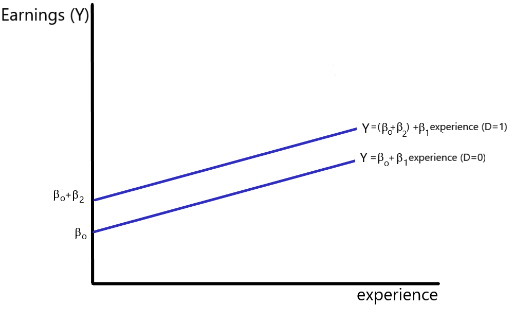
An inspection of equations 9.21 and 9.22 indicates that the intercept for the male population equals [latex]\beta_{0}+\beta_{2}[/latex] while the intercept for the female population simply equals [latex]\beta_{0}[/latex]. (The slope for both females and males equal [latex]\beta_{1}[/latex] under this specification.) This relationship is depicted in Figure 9.1.[13] The coefficient [latex]\beta_{2}[/latex] provides a measure of the difference between the female and male intercepts. A positive value of [latex]\beta_{2}[/latex] indicates that, ceteris paribus, males receive earnings that exceed those of females by an amount equal to [latex]\beta_{2}[/latex]. If [latex]\beta_{2}[/latex] is negative, male earnings are less than female earnings by an amount equal to [latex]\beta_{2}[/latex], holding work experience constant.
In general, when a dummy variable is included as a variable in a regression equation, the estimated coefficient provides a measure of the change in the dependent variable that occurs when the dummy variable equals one (as compared to the alternative where the dummy variable equals zero). To test to whether the presence of the qualitative variable alters the intercept, the appropriate hypotheses are:
H[latex]_0[/latex]: [latex]\beta_2=0[/latex]
and
H[latex]_1[/latex]: [latex]\beta _2\neq 0[/latex]
If the null hypothesis can be rejected at the preselected significance level, then it may be claimed that male earnings are significantly different than female earnings, controlling for the level of work experience. A simple two-tailed [latex]t[/latex] test can be used to test these hypotheses.
On the other hand, if you wished to determine whether male earnings are significantly greater than female earnings, a one-tailed test is appropriate. In this case, the hypotheses are:
H[latex]_{0}[/latex]: [latex]\beta_{2}\leq 0[/latex]
and
H[latex]_1[/latex]: [latex]\beta _{2}>0[/latex]
If the null hypothesis can be rejected at the preselected significance level, then it can be claimed that male earnings are significantly greater than female earnings (controlling for the level of work experience). Male-female earning differentials are examined in more detail in section 9.3.7.
Example: Earnings equation – difference in intercept
When the parameters of equation 9.20 are estimated using a sample of 4781 full-time workers who were participants in the National Longitudinal Study of the High School Class of 1972, the resulting equation is:[14]
\begin{equation}
\widehat{\text{earnings}}_{i}=\underset{(19.51)}{11,666}+\underset{(14.38)}{127.38}\text{experience}_{i}+\underset{(20.76)}{8873}D_{i} \tag{9.23}
\end{equation}
([latex]t[/latex]-statistics in parentheses)
This equation suggests that males, on average, earn $8873 more than females (in 1985 dollars), holding the level of recent work experience constant. The [latex]t[/latex]-ratio of 20.76 is significant at all conventional significance levels. If it is assumed that this model is correctly specified, then it may be concluded that male earnings are significantly greater than female earnings for individuals who have the same level of recent work experience.
It is likely, however, that there are a number of other important factors that affect earnings. These factors include: the respondent’s level of education, race, geographical location, and choice of occupation. As noted in Chapter 8, it is also more appropriate to use the natural log of earnings as the dependent variable and to include an (experience)[latex]^{2}[/latex] term as a regressor. A more complete earnings equation would take these factors into account. In fact, when these other variables are controlled for, the male-female earnings differential becomes substantially smaller.{[15] This serves as a reminder that regression coefficients serve as a measure of the effect of a change in the corresponding independent variable only if the model is correctly specified. (The issue of specification error is discussed in more detail in Chapter 10.)
Thus, equation 9.23 should be seen as an example of the use of dummy variables to measure the change in the intercept that results from the presence of a qualitative variable. It is not a definitive measure of male-female earning differentials.
9.3.2 Differences in slope
As noted above, a dummy variable is included as an additional regressor if it is believed that the presence of a qualitative variable results in a shift in the intercept of a regression equation. This implies that the qualitative variable represented by the dummy variable exhibits an impact that is independent of the effects of other independent variables. It is also quite possible, however, that the presence of a qualitative variable may alter the marginal effect resulting from a change in another independent variable. In other words, the qualitative variable may affect the magnitude of one or more of the slope coefficients in the equation.
Once again, a simple procedure can be used to determine whether a qualitative variable affects the magnitude of a slope coefficient. Suppose that an econometrician wishes to determine whether the effect of an additional unit of work experience on earnings differs between males and females. It is often argued, for example, that there is a “glass ceiling” that limits possibilities for promotions and pay increases for female workers. If this hypothesis is correct, an additional year of work experience will result in a larger increase in earnings for males than for females.
It was demonstrated above (in section 9.2) that an interaction term may be added to a regression equation to determine whether the level of one variable alters the marginal impact of another variable. In this case, we wish to examine whether the qualitative variable represented by the gender dummy variable alters the marginal impact of the work experience variable. Thus, it seems that it would be appropriate to include an interaction term that equals the product of the gender dummy variable and the experience variable. As before, the dummy variable, [latex]D_{i}[/latex] is defined as:
- D[latex]_{i}=1[/latex] if individual [latex]i[/latex] is male
- D[latex]_{i}=0[/latex] if individual [latex]i[/latex] is female
Let’s examine the effect of adding such an interaction term to a simple earnings equation:[16]
\begin{equation}
\text{earnings}_{i}=\beta_{0}+\beta_{1}\text{experience}_{i}+\beta_{2}( D_{i}\times \text{experience}_{i}) +u_{i} \tag{9.24}
\end{equation}
All of the variables in this equation are defined in the same manner as in equation 9.20.
For male respondents ([latex]D_{i}=1[/latex]), equation 9.24 reduces to:
\begin{equation*}
\text{earnings}_{i}=\beta _{0}+\beta _{1}\text{experience}_{i}+\beta _{2}( 1\times \text{experience}_{i}) +u_{i}
\end{equation*}
\begin{equation}
=\beta_{0}+( \beta_{1}+\beta _{2}) \text{experience}_{i}+u_{i} \tag{9.25}
\end{equation}
In the case of female respondents ([latex]D_{i}=0[/latex]), equation 9.24 reduces to:
\begin{equation*}
\text{earnings}_{i}=\beta_{0}+\beta _{1}\text{experience}_{i}+\beta _{2}( 0\times \text{experience}_{i}) +u_{i}
\end{equation*}
\begin{equation}
=\beta_{0}+\beta_{1}\text{experience}_{i}+u_{i} \tag{9.26} \end{equation}
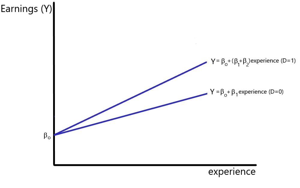
An examination of equations 9.25 and 9.26 indicates that the male and female earnings equations share the same intercept, but have different slopes. The slope of the population regression function for males equals [latex]\beta_{1}+\beta_{2}[/latex], while for females the slope simply equals [latex]\beta_{1}[/latex]. This relationship is depicted in Figure 9.2.
Male earnings increase at a rate that is significantly different from that of females if [latex]\beta_2[/latex] is significantly different than zero. This can be determined by performing a two-tailed test (using a standard [latex]t[/latex] test). A one-tailed hypothesis test can be used to determine whether male earnings grow at a rate that is significantly greater than that for female earnings.
Example: Earnings equation – difference in slope
To examine whether male and female earnings grow at different rates, the parameters of equation 9.24 were estimated using a sample of 4781 respondents from the National Longitudinal Study of the High School Class of 1972.[17] The estimated equation is:
\begin{equation}
\widehat{\text{earnings}}_{i}=\underset{(28.29)}{16,158}+\underset{(5.79)}{57.40}\text{experience}_{i}+\underset{(20.07)}{134.16}\left( D_{i}\times \text{experience}_{i}\right) \tag{9.27}
\end{equation}
([latex]t[/latex]-statistics in parentheses)
Since the estimated coefficient on the interaction term is significantly greater than zero, these results suggest that male earnings increase more rapidly than female earnings as work experience increases. In particular, these results indicate that an additional month of recent work experience increases annual female earnings by $57.40. The annual earnings of males, however, appear to increase by $191.56 ($57.40 + $134.16) for each additional month of work experience.
As noted above, this model specification assumes that the intercept for males and females is the same. It is quite possible that both the intercept and slope coefficients differ between males and females. This possibility is discussed in section 9.3.6. Once again, it should be noted that a more complete specification would include such factors as educational attainment, race, geographical location, occupational choice, and the nonlinearity of the earnings-experience relationship.
The return to beauty
Labor economists have long used dummy variables to capture the effect of qualitative variables on individual earnings. For example, dummy variables for race, gender, marital status, and geographical location are typically included in estimated earnings equations. Recently, however, Hamermesh and Biddle (1994), have taken this process one step further by examining the effect of appearance on earnings.
Hamermesh and Biddle found that those individuals who are considered to be below average in appearence are paid 5% to 14% less than those who are considered to be of average appearance. Those whose appearance is considered to be above average are paid 6% to 13% more than those considered to be average. These results appear to hold for both men and women (slightly higher coefficients were found for males). Less attractive women, however, also tend to have lower labor force participation rates and marry less educated men.
9.3.3 Dummy variables in practice
In determining the specification of an econometric model, an econometrician must determine whether qualitative variables should be included as additional regressors or through the use of interaction terms. Quite often, the underlying economic model will generate predictions about whether the presence or absence of a qualitative variable will affect the intercept or slope parameters. Under these circumstances, it is easy to determine how the dummy variable should be entered. When economic theory does not generate such predictions, however, the choice becomes more difficult. If it is believed that the characteristic represented by the dummy variable directly affects the dependent variable, then the dummy variable should be included as a separate independent variable. If, however, it is anticipated that the underlying qualitative variable alters the effect of some other variable, then an interaction terms should be included to investigate this hypothesis.
In many applications, several dummy variables are included in regression equations to capture the effect of a variety of qualitative variables. For example, when estimating earnings equations, an econometrician may wish to include a set of dummy variables representing alternative levels of educational attainment. The same equation may also contain dummy variables for race, gender, or marital status. In time-series models based on monthly or quarterly data, monthly or quarterly dummy variables may also be included to account for the seasonal fluctuations that occur in many economic phenomena.
Let’s examine how a set of dummy variables can be included into a regression model.
Economic Literacy of High School Students
Walstad and Soper (1988) used data from a large nationally representative sample to examine determinants of the level of economic literacy among high school students. The level of economics literacy was measured through the use of the Test of Economic Literacy, a nationally normed exam that is often used to measure the level of economic literacy among high school students. The independent variables included in this model capture the effect of student characteristics (such as IQ, race, gender, and senior class standing), teacher characteristics (such as the number of college economics credit hours undertaken by the teacher), course characteristics (dummy variables representing economics courses, consumer economics courses, and social science courses), and school characteristics (such as geographical location, and size of the school).
It was found that, on average, the overall level of economic literacy among high school students was quite low. The educational background of the teacher was, not surprisingly, an important determinant of student performance on this exam. Students performed significantly better when their teachers had previous training in economics and participated in teacher training workshops.
This study represents an interesting example of how dummy variables can be used to examine the quality of educational programs. The results of this study (and several related studies) were used by the Joint Council on Economic Education to convince several states to introduce mandatory economics components in their high school social studies curriculum.
9.3.4 Example: Earnings and educational attainment
Participants in the National Longitudinal Survey of the High School Class of 1972 may be separated into the following levels of educational attainment: high school degree, 1-3 years of college, bachelor’s degree, master’s degree, or a Ph.D. or equivalent degree. A set of educational dummy variables can be constructed corresponding to these alternative levels of educational attainment.
Is there a “sheepskin effect?”
In general, econometricians use qualitative variables when quantitative variables are not available. Typically, for example, it is better to include an “income” variable measured in quantitative terms than to include dummy variables representing “low,” “middle,” or “high” incomes.
In the case of educational attainment, however, there is some evidence suggesting that the level of educational attainment (as represented by a set of dummy variables representing alternative levels of educational attainment) may be more important that “years of education.” A recent study by Grubb (1993), for example, finds that individuals who enroll in postsecondary education but do not complete an associate’s or bachelor’s degree have earnings that are not significantly different from the earnings of high school graduates.
One problem with using “years of education” as a quantitative variable is that 16 years of education might result in very different levels of educational attainment for different people. Many economists argue that the presence of a college degree (the “sheepskin effect”) provides more information to potential employers than the length of time spent in educational institutions. Grubb’s result suggests that, in specifying earnings equations, a set of educational attainment dummy variables provides a more appropriate measure of education than a “years of education” variable. An example of the use of educational attainment dummy variables for this purpose appears in equation 9.28.
| Variable Name | Description |
|---|---|
| earnings[latex]_i[/latex] |
= total earnings of individual i in 1985 (in dollars) |
| experience[latex]_i[/latex] |
= total months of work experience at 2 most recent jobs |
| SC[latex]_i[/latex] |
= 1 if the individual has completed 1-3 years of college; = 0 otherwise |
| CD[latex]_i[/latex] |
= 1 if the individual’s highest level of education is a bachelor’s degree, = 0 otherwise |
| MA[latex]_i[/latex] |
= 1 if the individual’s highest level of education is a master’s degree, = 0 otherwise |
| PhD[latex]_i[/latex] |
=1 if the individual has acquired a Ph.D., M.D., J.D, or similar degree, = 0 otherwise |
To measure the effect of educational attainment on earnings, an expanded earnings equation may be specified as:
\begin{equation}
\text{earnings}_{i}=\beta_{0}+\beta _{1}\text{experience}_{i}+\beta _{2}( \text{experience}_{i} ^{2}+\beta _{3}\text{SC}_{i}\tag{9.28}
\end{equation}
\begin{equation*}
+\beta _{4}\text{CD}_{i}+\beta _{5}\text{MA}_{i}+\beta _{6}\text{PhD}_{i}+u_{i}
\end{equation*}
The variables used in this equation are defined in Table 9.1. Notice that the dummy variable corresponding to a high school education has been excluded from the set of dummy variables appearing in equation 9.28. This was not an oversight. Suppose that a dummy variable was included that corresponded to a high school degree. For each individual in this sample, one and only one dummy variable would equal one;[18]} all other dummy variables have a value equal to zero.
Consider the summation defined as:
SUM = HS + SC + CD + MA + PHD
This linear combination of these dummy variables equals one for each and every observation (since one and only one of these cases holds for each respondent).
As noted in Chapter 6, an econometric model cannot be estimated when one of the right-hand side variables can be written as a linear combination of the other variables. If all possible levels of educational attainment were included in equation 9.28, the constant term would equal an exact linear combination of the set of educational attainment dummy variables. If an attempt were made to estimate the parameters of a model in which each of these educational attainment dummy variables are included, the regression package would report that it is unable to estimate the parameters of the equation. This is an example of a phenomenon known as the dummy variable trap. To avoid this problem, one of these educational attainment variables has to be omitted from the regression equation.
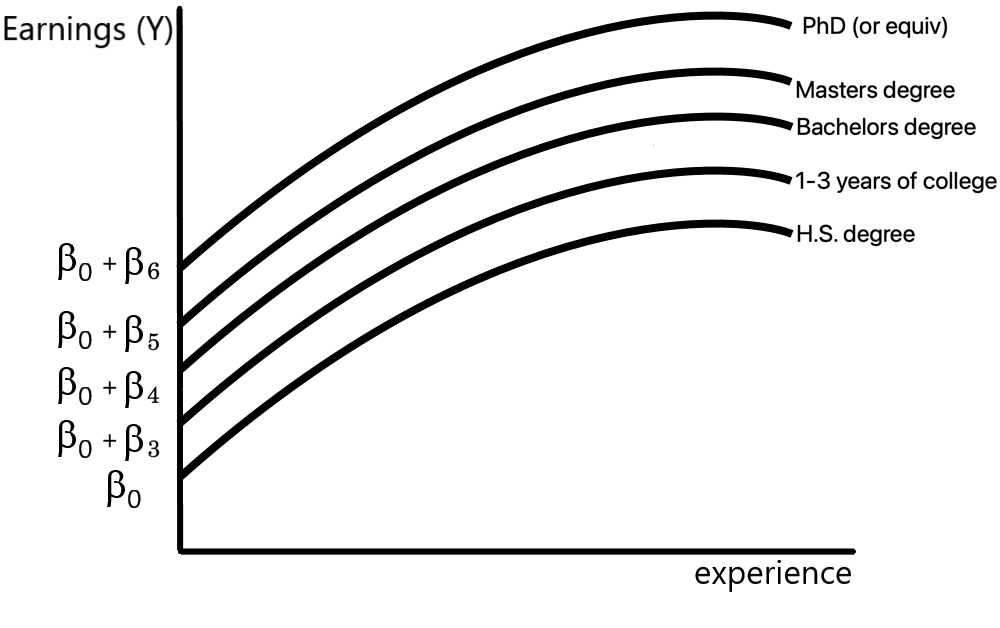
Does the absence of a dummy variable present a problem in interpreting an estimated version of equation 9.28? The strategy used above to determine the difference between the intercepts of male and female earnings equations can be applied here. For individuals that have completed only a high school degree, the value of all of the educational attainment dummy variables in this equation equal zero. The intercept for these individuals simply equals [latex]\beta_{0}[/latex]. For those individuals who have completed 1-3 years of college, the intercept equals [latex]\beta_{0}+\beta _{3}[/latex]. The intercepts for the subsamples corresponding to each level of educational attainment are given in Table 9.2. Notice that each of the coefficients multiplying the dummy variables provides a measure of the increase in earnings that results from the specified level of education as compared to the earnings of a high school graduate. [19]
| Level of Education | Intercept |
|---|---|
| H.S. Degree | [latex]\beta_0[/latex] |
| 1-3 Years of college | [latex]\beta_0+\beta_3[/latex] |
| Bachelors degree | [latex]\beta_0+\beta_4[/latex] |
| Masters degree | [latex]\beta_0+\beta_5[/latex] |
| Ph.D. (or equivalent) | [latex]\beta_0+\beta_6[/latex] |
This relationship is represented in Figure 9.3. (Note that the earnings-experience curve is nonlinear due to the inclusion of the experience[latex]^{2}[/latex] term.)
When the parameters of equation 9.28 are estimated using a sample consisting of 4781 full-time workers, the estimated sample regression function is:
\begin{equation}
\widehat{\text{earnings}_{i}}=\underset{(11.38)}{10,326}+\underset{(6.16)}{237.68}\text{experience}_{i}-\underset{(-2.20)}{0.833}\left( \text{experience}_{i}\right) ^{2} \tag{9.29} \end{equation}
\begin{equation*}
+\underset{(2.39)}{1,374}\text{SC}_{i}+\underset{(10.89)}{5,727}\text{CD} _{i}+\underset{(8.52)}{6,556}\text{MA}_{i}+\underset{(18.16)}{19,799}\text{PhD}_{i}
\end{equation*}
(t-statistics in parentheses)
Note that each of the coefficients in equation 9.29 is significantly different than zero at the .05 significance level. As noted in Chapter 8, a positive and large coefficient on the “experience[latex]_{i}[/latex]” variable combined with a negative and small coefficient on the “experience[latex]_{i}^{2}[/latex]” variable is consistent with an inverted-U shaped relationship between work experience and the level of earnings.
This estimated equation suggests that education beyond the high school level results in a significant increase in earnings. In particular, these results indicate that individuals with 1-3 years of college earn, on average, $1,374 more per year (in 1985 dollars) than an individual with a high school degree, holding work experience constant. In a similar manner, equation 9.29 indicates that individuals with bachelor’s, master’s, or Ph.D. (or equivalent) degrees receive, on average, $5,727, $6,556, and $19,799 more than high school graduates who possess the same level of work experience.
Once again, it should be noted that a more appropriate specification for an earnings equation would take gender, race, and geographical location into account. This example is provided primarily to illustrate how a set of dummy variables may be used to represent all of the possible values for a qualitative variable, such as educational attainment.
9.3.5 Caution: The dummy variable trap
The dummy variable trap discussed above is a problem often experienced by beginning econometricians. It will be experienced whenever an attempt is made to estimate a model that includes a constant term and a set of dummy variables that provides categories for each and every possible outcome in the sample. When an econometrics software package is faced with a model of this sort it will respond with a message that resembles one or more of the following:
- matrix cannot be inverted;
- a perfect multicollinearity problem exists;
- matrix is singular; and/or
- parameter estimates cannot be formulated.
If you are working with dummy variables and a message of this sort appears, it is likely that the dummy variable trap has occurred. The simplest solution is to omit one possible case for each type of dummy variable.[20] Thus, when an intercept term is included in a cross-sectional or panel data regression, the independent variables cannot include dummy variables for both genders, all levels of marital status, all races, all types of geographical location, all religious groupings, etc. In time series studies, regression equations cannot include dummy variables for all possible time periods.
An alternative solution to the dummy variable problem is to omit the constant term but include dummy variable for each possible outcome. For example, the following (simplified) earnings equation could be estimated:
\begin{equation}
\ln (\text{earnings}_{i}\text{) = }\beta_{1}\text{Male}_{i}+\beta _{2}\text{Female}_{i}+\beta _{3}\text{experience}_{i}+u_{i} \tag{9.30} \end{equation}
For males, the variable Male[latex]_{i}[/latex] always equals one and the variable Female[latex]_{i}[/latex] always equals zero. Thus, equation 9.30 simplifies to:
\begin{equation*}
\ln (\text{earnings}_{i}\text{) = }\beta _{1}+\beta _{3}\text{experience} _{i}+u_{i}
\end{equation*}
For females, equation 9.30 simplifies to:
\begin{equation*}\ln (\text{earnings}_{i}\text{) = }\beta_{2}+\beta_{3}\text{experience}_{i}+u_{i}
\end{equation*}
As this example indicates, when a constant term is omitted and dummy variables are included for each possible outcome, the coefficient on each dummy variable represents the intercept for the subsample possessing the characteristic represented by the dummy variable. This solution works, however, only if there is a dummy variable problem with a single set of dummy variables. If dummy variables for each possible level of educational attainment were added to equation 9.30, perfect multicollinearity would still occur.[21] In practice, though, it is a much more common practice to omit a dummy variable corresponding to one possible outcome than to omit the constant term in a regression.
How do you decide which dummy variable to omit when you are faced with a set of dummy variables representing mutually exclusive alternatives? One common practice is to exclude the dummy variable for a category that represents the largest number of cases. In this case, the intercept in the equation represents the “usual” intercept, while the dummy variables representing less commonly observed outcomes allow for deviations from this “usual” case. For example, when dealing with qualitative independent variables representing health status, it is common to omit a variable representing “good health” while including one or more dummy variables for those individuals who report health problems.
In general, however, there is no simple rule that indicates which dummy variable should be omitted. If, for example, an econometrician uses a set of monthly dummy variables to capture seasonal patterns in the level of a dependent variable, there is no logical reason to select any particular month to omit. Fortunately, however, the choice of which dummy variable to omit does not really matter very much. No matter which dummy variable is omitted from the regression equation, the estimated coefficients and [latex]t[/latex]-ratios for all of the continuous variables in the regression equation will be the same.[22]
9.3.6 Chow test
One interesting application of the use of dummy variables involves testing to determine whether the parameters of a regression equation are the same in two subsamples. For example, an econometrician may wish to determine whether male and female earning equations should be estimated separately or jointly.In a similar manner, a macroeconomist may wish to determine whether a trade agreement (or other event) has altered the structural parameters of a consumption function.
The classical regression model is based upon the assumption that the equation governing the relationship between the dependent and independent variables is the same for all observations. It is inappropriate to estimate a relationship based upon all observations if the parameters are different for some observations. On the other hand, if the same relationship holds for all observations, it is inefficient to estimate separate equations for different subsamples. If it is believed that it is likely that different structural relationships hold in two or more subsamples, the appropriate solution is to test whether the parameters are in fact different in these subsamples. A test of this type is referred to as a Chow test in honor of its developer, Gregory Chow.[23] Let’s consider a simple example.
Suppose that we wish to determine whether the parameters of equation 9.28 are significantly different for males and females. The discussion in section 9.3.1 suggests that we can test for a difference in intercept by including a gender dummy variable as an additional regressor. As noted in section 9.3.2, differences in slope coefficients may be investigated through the use of an interaction term that equals the product of the gender dummy variable and the corresponding independent variable. This suggests that we can determine whether all of the parameters are different by including a gender dummy variable and interaction terms between a gender dummy variable and each of the independent variables. This relationship may be expressed as:
\begin{equation}
\text{earnings}_{i}=\beta_{0}+\beta_{1}\text{experience}_{i}+\beta_{2}\left( \text{experience}_{i}\right)^{2}+\beta_{3}\text{SC}_{i} \tag{9.31}
\end{equation}
\begin{equation*}
+\beta _{4}\text{CD}_{i}+\beta _{5}\text{MA}_{i}+\beta_{6}\text{PhD} _{i}+\beta _{7}D_{i}
\end{equation*}
\begin{equation*}
+\beta _{8}\left( D_{i}\times \text{experience}_{i}\right) +\beta _{9}\left( D_{i}\times \text{experience}_{i}^{2}\right) +\beta _{10}\left( D_{i}\times \text{SC}_{i}\right)
\end{equation*}
\begin{equation*}
+\beta_{11} ( D_{i}\times \text{CD}_{i} ) +\beta _{12} ( D_{i}\times \text{MA}_{i} ) +\beta_{13}( D_{i}\times \text{PhD}_{i})+u_{i}
\end{equation*}
where: D[latex]_{i}[/latex] is a dummy variable equal to one for male respondents and equal to zero for females.
To determine whether male and female earnings equations are significantly different, it is necessary to test the hypotheses:
H[latex]_0[/latex]: [latex]\beta _7=\beta _8=\cdots =\beta _{13}=0[/latex]
and
H[latex]_1[/latex]: at least one of the coefficients [latex]\beta _7,\beta _8,\ldots ,\beta _{13}[/latex] is not equal to zero
These hypotheses may be tested using the [latex]F[/latex]-test discussed in Chapter 7. This procedure involves:
- Step 1: Select a significance level that is appropriate taking into account the probabilities of Type I and Type II errors.
- Step 2: Formulate two versions of the regression model: an unrestricted version that does not impose any restrictions on the parameter values; and a restricted version that imposes the restrictions embodied in the null hypothesis. The unrestricted model appears in equation 9.31. The restricted model is formulated by setting the parameters [latex]\beta _7,\beta _8,\ldots,\beta_{13}[/latex] equal to zero. (The restriction that is imposed here is that the coefficients of the earnings equation are the same for male and female respondents.) This results in an equation in which all terms involving the dummy variable are omitted. An alert reader will note that the restricted model is equivalent to equation 9.28.
- Step 3: Estimate the parameters of the unrestricted version of the model. Define ESS[latex]_{u}[/latex] as the error sum of squares (= [latex]\sum \hat{u}_{i}^{2}[/latex]) in the unrestricted model.[24]
- Step 4: Estimate the parameters of the restricted version of the model. Define ESS[latex]_r[/latex] as the error sum of squares in the restricted model.
- Step 5: Formulate the statistic: \begin{equation}
F=\frac{(\text{ESS}_r-\text{ ESS}_u\text{) / }m}{\text{ESS}_u\text{ / [}N-(k+1)]} \tag{9.32}
\end{equation}
where [latex]m[/latex] is the number of linear restrictions imposed by the null hypothesis, [latex]N[/latex] is the number of observations (in the entire sample), and [latex]k+1[/latex] is the number of parameters in the unrestricted model (=14 in this example). This statistic is distributed as an [latex]F[/latex] statistic with [latex]m[/latex] and [latex]N-(k+1)[/latex] degrees of freedom for the numerator and denominator respectively. - Step 6: Reject the null hypothesis if the estimated [latex]F[/latex] statistic exceeds the critical value at the preselected significance level.
When the parameters of equation 9.31 are estimated, the resulting equation is:
\begin{equation}
\widehat{\text{earnings}}_{i}=\underset{(5.57)}{7072}+\underset{(4.58)}{261.95}\text{experience}_{i}-\underset{(-2.77)}{1.59}( \text{experience} _{i}) ^{2} \tag{9.33} \end{equation}
\begin{equation*}
+\underset{(2.47)}{2044}\text{SC}_{i}+\underset{(6.86)}{5275}\text{CD}_{i}+\underset{(5.72)}{6279}\text{MA}_{i}+\underset{(10.28)}{20,007}\text{PhD}_{i} \end{equation*}
\begin{equation*}
+\underset{(3.63)}{6346}D_{i}-\underset{(-0.23)}{17.08}(D_{i}\times \text{experience}_{i})
\end{equation*}
\begin{equation*}
+\underset{(1.00)}{0.74}(D_{i}\times \text{experience}_{i}^{2}) – \underset{(-0.67)}{743}( D_{i}\times \text{SC}_{i}) +\underset{(1.02)}{1034}( D_{i}\times \text{CD}_{i}) \end{equation*}
\begin{equation*}
+\underset{(0.79)}{1167}( D_{i}\times \text{MA}_{i} ) -\underset{(-0.90)}{2082}( D_{i} \times \text{PhD}_{i}) \end{equation*}
\begin{equation*}
\text{(}t\text{-ratios in parentheses)} \end{equation*}
The error sum of squares (ESS[latex]_{u}[/latex]) in this equation is [latex]0.9203 \times 10^{12}[/latex]. In the restricted version of this model, the error sum of squares (ESS[latex]_{r}[/latex]) equals [latex]1.007 \times 10^{12}[/latex]. The resultant [latex]F[/latex] statistic is: \begin{equation*}
F=\frac{(\text{ESS}_{r}-\text{ ESS}_{u}\text{) / }m}{\text{ESS}_{u}/[N-(k+1)]}
\end{equation*}
\begin{equation*}
=\frac{(1.007-\text{ 0.9203) / 7}}{0.9203/[4781-(13+1)]} \end{equation*}
\begin{equation*}
=64.17
\end{equation*}
Since this statistic exceeds the critical value at all conventional significance levels, it can be concluded that one or more of the coefficients in the earnings equation for males is significantly different than the corresponding coefficient(s) for females. In particular, an inspection of the [latex]t[/latex]-ratios in equation 9.33 suggests that the difference between male and female earnings equation is primarily due to a difference in the intercept. This indicates that an appropriate specification of an earnings equation should include a gender dummy variable as an independent variable to allow for a difference in the intercept.
9.3.7 Example: Male-female earnings differentials
To investigate male-female earnings differentials, it is useful to specify a more elaborate earnings equation that takes into account the major factors that affect individual earnings. These factors include the individual’s work experience, educational attainment, geographical location, race, and gender. Let’s examine such a model.
As noted in Chapter 8, earnings equations are generally specified in log-linear form. Table 9.3 contains a listing of the specific variables that are included in this earnings equation. When a large number of variables are included in a regression equation, the results are generally reported in tabular, rather than equation, form. Table 9.4 contains the parameter estimates and [latex]t[/latex]-ratios for the log-earnings equation.
| Variable name | Description |
|---|---|
| earnings |
= total earnings of individual i in 1985 (in dollars) |
| experience |
= number of months worked at two most recent jobs |
| experience[latex]^2[/latex] |
= experience [latex]\times[/latex] experience |
| SC |
= 1 if the individual has completed 1-3 years of college; – 0 otherwise |
| CD |
= 1 if the individual’s highest level of education is a bachelor’s degree; = 0 otherwise |
| MA |
= 1 if the individual’s highest level of education is a master’s degree; = 0 otherwise |
| PHD |
= 1 if the individual has acquired a Ph.D., M.D., J.D, or similar degree; = 0 otherwise |
| NE |
= 1 if the individual lived in the northeast; = 0 otherwise |
| SOUTH |
= 1 if the individual lived in the south; = 0 otherwise |
| BLACK |
= 1 if the individual is African-American; = 0 otherwise |
| ASIAN |
= 1 if the individual is Asian-American; = 0 otherwise |
| HISPANIC |
= 1 if the individual is Hispanic; = 0 otherwise |
| FEMALE |
= 1 if the individual is female; =0 otherwise |
| *significant at the .05 level | ||
| ** significant at the .01 level | ||
| Variable name | Estimated coefficients | [latex]t[/latex]-ratio |
|---|---|---|
| constant | 9.208 | 217.16** |
| experience | 0.018 | 10.56** |
| experience[latex]^2[/latex] | -0.00009 | -5.36** |
| SC | 0.108 | 4.23** |
| CD | 0.265 | 11.34** |
| MA | 0.341 | 9.97** |
| PHD | 0.627 | 12.93** |
| NE | 0.071 | 2.96** |
| SOUTH | -0.014 | -0.60 |
| BLACK | -0.103 | -3.07** |
| ASIAN | 0.147 | 1.56 |
| HISPANIC | 0.034 | 0.76 |
| FEMALE | -0.419 | -21.92** |
Notice that this model contains four sets of dummy variables: educational attainment (SC, CD, MA, and PhD), geographical location (NE and SOUTH), race (BLACK, ASIAN, and HISPANIC), and gender (FEMALE). To avoid a dummy variable trap, one possible outcome is omitted from each of these categories. In the case of educational attainment, the omitted category (as before), corresponds to a high school degree. Thus, for example, the coefficient of 0.265 on the CD variable indicates that, on average, an individual in this sample possessing a B.A. or B.S. degree earned 26.5% more in 1986 than individuals who possess a high school degree (holding other variables constant).
The omitted category for geographical location includes the midwestern and western states. Thus, the results in Table 9.4 indicate that earnings are, on average, 7.1% higher in the northeast than in the midwestern and western U.S. These estimates also suggest that there is no significant difference between the earnings in the southern states and those in the midwestern and western states.
Since the excluded racial category corresponds to white individuals, the estimates in Table 9.4 suggest that. African-American workers, on average, earn 10.3% less than white workers. Hispanic and Asian-American workers, however, have earnings that are not significantly different than the earnings of white workers.
These results also suggest that the earnings of full-time female workers are, on average, 41.9% less than the earnings of full-time male workers, holding other variables constant.
9.3.8 Piecewise linear models
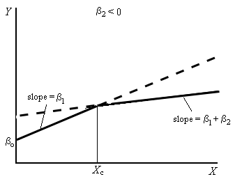
Dummy variables may also be used to estimate models that are piecewise linear. A piecewise linear model is one in which the regression relationship consists of two or more linear segments. Examples of piecewise linear relationships appear in Figure 9.4. In the two cases illustrated in this figure, a structural change occurs when the independent value ([latex]X[/latex]) exceeds some threshold value ([latex]=X_{c}[/latex]). The independent variable is often simply a trend variable (with successive values defined as [latex]1, 2, \ldots, N[/latex]). More complex models may have more than one such segment.
Piecewise linear models are also sometimes referred to as spline functions or jackknife models (since the graph resembles an open jackknife).
To represent the piecewise linear relationships of the type illustrated in Figure 9.4, it is necessary to define a dummy variable, [latex]D_{i},[/latex] as:
[latex]D_{i}=1[/latex] if [latex]X_{i}\geq X_{c}[/latex]
[latex]D_{i}=0[/latex] if [latex]X_{i}\lt X_{c}[/latex]
The piecewise linear model can be specified as: \begin{equation}
Y_{i}=\beta_{0}+\beta_{1}X_{i}+\beta_{2}D_{i}(X_{i}-X_{c})+u_{i} \tag{9.34}
\end{equation}
For those observations at which the value of the independent variable [latex]X[/latex] is less than [latex]X_{c}[/latex], the regression relationship is: \begin{equation*}
Y_{i}=\beta_{0}+\beta _{1}X_{i}+u_{i}
\end{equation*}
since ([latex]D_{i}=0[/latex]). For the observations at which[latex]X_{i}\geq X_{c}[/latex] ([latex]D_{i}=1[/latex]), the relationship is:
\begin{equation*}
Y_{i}=( \beta_{0}-\beta _{2}X_{c}) +( \beta _{1}+\beta _{2}) X_{i}+u_{i}
\end{equation*}
Thus, at point [latex]X_{c}[/latex], the regression relationship shifts from a linear segment with a slope of [latex]\beta_{1}[/latex] to another linear segment that has a slope equal to [latex]\beta_{1}+\beta_{2}[/latex]. (The intercept of the first segment equals [latex]\beta_{0}[/latex] while the intercept of the second segment is [latex]\beta_{0}-\beta _{2}X_{c}[/latex].) Note that when [latex]\beta_{2}[/latex] is negative, the slope becomes flatter for values of [latex]X_{i}[/latex] that exceeds the threshold value [latex]X_{c}[/latex]. A positive value of [latex]\beta_{2}[/latex], however, indicates that the function becomes steeper when [latex]X_{i}[/latex] exceeds the threshold value of [latex]X_{c}[/latex].
9.3.9 Example: Profitability of aerospace firms
Piecewise linear models are often used to determine whether the trend growth of some economic variable has changed because of an event occurring at a particular point in time (or over some interval of time). Poirier and Garber (1974) provide an interesting example of such a model in a study of the profitability of aerospace firms during the years 1951-71. This study used a piecewise linear model in which the time trend of profits for each firm was represented by three linear segments corresponding to the periods 1951-54, 1954–65, and 1965-71. A simplified version of their model can be expressed as:\footnote{%
The full model used by Poirier and Garber included 12 additional independent variables (various measures of Department of Defense expenditures, and a collection of dummy variables representing the individual firms in the sample). The sample included information for 9 firms measured over a 21-year period. Because of missing data (due to mergers or changes in the mix of products produced by these firms), the sample contains 119 observations (they also analyze a smaller sample containing 112 observations). Note that there would have been 189 observations if data had been available on all firms in each year.}
\begin{equation}
\text{Profit Rate}_{it}=\beta_{0}+\beta_{1}\text{Year}_{t}+\beta_{2}[ \text{Peacetime}_{t}\times (\text{Year}_{t}-4) ]\tag{9.35}
\end{equation}
\begin{equation*}
+\beta _{3}[ \text{Vietnam}_{t}\times ( \text{Year}_{t}-15) ] +u_{it}
\end{equation*}
where:
- Profit Rate[latex]_{it}[/latex] = profit rate (= total profits / total assets) for firm [latex]i[/latex] in year [latex]t[/latex].
- Year[latex]_t[/latex] = # of years since 1950.
- Peacetime[latex]_t[/latex] = 1 during the peacetime years (4 < Year[latex]_t[/latex] < 15) (= 0 otherwise).
- Vietnam[latex]_t[/latex] =during the Vietnam War years (15 < Year[latex]_t[/latex] < 19) (= 0 otherwise).
- [latex]u_{it}[/latex] = random error term for firm [latex]i[/latex] in year [latex]t[/latex].
The dual subscripts on the Profit[latex]_{it}[/latex] and[latex]u_{it}[/latex] variables indicate that this is pooled data. This model was estimated using a sample involving 9 firms over 19 years ([latex]t=1,19[/latex]). In each year, there are at most 9 observations (fewer observations exist in some years because of missing data).
Notice that equation 9.35 is a generalization of the basic spline function appearing in equation 9.34. Under this specification:
- [latex]\beta_{2}[/latex] is a measure of the annual change in the profit rate during the Korean War (1951-54),
- [latex]\beta _{3}[/latex] is a measure of the annual change in the profit rate during the peacetime years (1954-65), and
- [latex]\beta_{4}[/latex] is a measure of the annual change in the profit rate during the Vietnam War years (1965-1971).A[25]
When Poirier and Garber estimated their model, they found that the estimated parameters corresponding to [latex]\beta_{1}[/latex] and [latex]\beta_{3}[/latex] were significant and positive. The estimated coefficient corresponding to [latex]\beta_{2}[/latex] was negative and significant. Thus, their estimates suggest that the profit rate for these aerospace firms increased significantly during both the Korean War and the Vietnam War periods. Profit rates, however, declined for these firms during the peacetime years.
9.4 Summary
In this chapter, a number of useful econometric tools have been discussed. These tools greatly expand the range of models that can be investigated by econometricians. Interaction terms make it possible to analyze the joint impact of two or more economic variables on a dependent variable. Econometricians use dummy variables to investigate the impact of qualitative independent variables in a regression framework. Dummy variables may also be used to test for the existence of structural change in an econometric relationship.
The use of these techniques make it possible for econometric models to more accurately reflect real-world economic processes.
9.5 Key Concepts
- interaction effects
- qualitative variables
- dummy variables
- dummy variable trap
- Chow test
- piecewise linear model
- spline function
9.6 Exercises and problems
- Use the formulas for OLS estimators appearing in Chapter 4, to show that the relationships appearing in equation system 9.7 will always hold.
- Use the data in the file “cons.dat” to estimate the parameters of the consumption function:
\begin{equation*}
\text{C}_{t}=\beta _{o}+\beta _{1}\text{YD}_{t}+u_{t} \end{equation*}- when both C[latex]_{t}[/latex] and YD[latex]_{t}[/latex] are expressed in billions of dollars (as in the original table).
- when C[latex]_{t}[/latex] is converted into a measure expressed in millions of dollars, but YD[latex]_{t}[/latex] is expressed in billions (e.g., create a transformed consumption variable by multiplying C[latex]_{t}[/latex] by 1,000). How do the new intercept and slope parameters compare with those estimated in part (a)?
Have the [latex]t[/latex]-ratios changed? - when C[latex]_{t}[/latex] is expressed in billions of dollars, but YD[latex]_{t}[/latex] is expressed in millions of dollars. How do the new intercept and slope parameters compare with those estimated in part (a)? Have the [latex]t[/latex]-ratios changed?
- when both C[latex]_{t}[/latex] and YD[latex]_{t}[/latex] are expressed in millions of dollars. How do the new intercept and slope parameters compare with those estimated in part (a)? Have the [latex]t[/latex]-ratios changed?
- In some applications, economists wish to examine the relative importance of alternative variables on the level of the dependent variable in a regression model. The magnitude of the slope coefficients in a simple OLS regression cannot be used for this comparison since the magnitude of these coefficients are affected by the units in which each independent variable is measured. Such a comparison, however, is sometimes made by constructing standardized regression coefficients. To estimate standardized regression coefficients, each of the independent variables in the regression model is transformed by using the relationship: \begin{equation*}
\widetilde{X}_{ji}=\frac{X_{ji}-\overline{X_{j}}}{\hat{\sigma}_{X_{j}}} \end{equation*}
where: [latex]\overline{X}_{j}[/latex] equals the sample mean of [latex]X_{ji}[/latex] and [latex]\hat{\sigma}_{X}[/latex] is the sample standard deviation for [latex]X_{ji}[/latex]. The standardized regression coefficients are calculated by performing an OLS regression of [latex]Y_{i}[/latex] on the transformed independent variables ([latex]\widetilde{X}_{1},\ldots , \widetilde{X}_{j}[/latex]).- What will be the sample mean and standard deviation for each of the transformed independent variables?
- What is the interpretation of the slope coefficients in this model? Why might they be considered standardized regression coefficients?
- An econometrician specifies the following regression model: \begin{equation*}
\text{GPA}_{i}=\beta _{0}+\beta _{1}\text{SAT}_{i}+\beta _{2}\text{StudyHrs} _{i}+\beta _{3}\left( \text{SAT}_{i}\times \text{StudyHrs}_{i}\right) +u_{i} \end{equation*}
Interpret the meaning of the parameter [latex]\beta_{3}[/latex]. What would a positive value for [latex]\beta_{3}[/latex] imply? What would be implied by a negative value of [latex]\beta _{3}[/latex]? - An econometrician specifies the following demand equation for compact discs (CDs[latex]_{i}[/latex]):
\begin{equation*}
\text{CDs}_{i}=\beta _{0}+\beta _{1}\text{Price}_{i}+\beta _{2}\text{Income}_{i}+\beta _{3}\left(\text{Price}_{i}\times \text{Income}_{i}\right) +u_{i} \end{equation*}
where: Price[latex]_{i}[/latex] = price of CDs facing person [latex]i[/latex], and Income[latex]_{i}[/latex] = income of person [latex]i[/latex]. What does the parameter [latex]\beta_{3}[/latex] represent? Is this likely to be positive or negative? Explain. - Hamermesh and Soss (1974) discuss the economic determinants of suicide rates. Using aggregate data (pooled time-series and cross-section data) on males aged 20-64, they estimate the following equation: \begin{equation*}
\text{\^{S}}_{t}=\underset{(5.29)}{26.54}-\underset{(-5.82)}{7.73}\text{YPL} _{t}+\underset{(6.20)}{0.56}\text{YPL}_{t}^{2}-\underset{(-2.86)}{2.08}\text{Age}_{t}+\underset{(3.73)}{0.065}\text{Age}_{t}^{2} \end{equation*}
\begin{equation*}
-\underset{(-3.62)}{0.0005}\text{Age}_{t}^{3}-\underset{(-3.15)}{70.16}\text{UN}_{t}+\underset{(5.68)}{3.40}\left( \text{UN}_{t}\cdot \text{Age} _{t}\right)
\end{equation*}
\begin{equation*}
\text{(}t\text{-statistics in parentheses)} \end{equation*}
where:- S[latex]_t[/latex] = suicide rate at time [latex]t[/latex] (suicides / 100,000 population).
- YPL[latex]_t[/latex] = a measure of the discounted value of future permanent income at time [latex]t[/latex].
- Age[latex]_t[/latex] = age (in years) of individuals in cohort at time [latex]t[/latex].
- UN[latex]_t[/latex] = unemployment rate at time [latex]t[/latex] (expressed as a fraction, not a percentage)
- Why is an interaction term between UN[latex]_{t}[/latex] and Age[latex]_{t}[/latex] included?
- What does the positive coefficient on this interaction term suggest?
- Would an increase in the unemployment rate raise or lower suicide rates for 25 year old individuals? Explain.
- Is the effect of an increase in the unemployment rate larger or smaller effect for 35 year old individuals than for 25 year old males? Explain.
- When the variables [latex]Y_{i}[/latex] and [latex]X_{i}[/latex] are measured in thousands of dollars, an estimated regression equation is given by: \begin{equation*}\hat{Y}_{i}=\underset{(2.85)}{1.41}+\underset{(4.16)}{0.967}X_{i} \end{equation*}Determine the estimated equation and [latex]t[/latex]-ratios that would occur if Y[latex]_{i}[/latex] and X[latex]_{i}[/latex] were measured in terms of dollars (instead of thousands of dollars).
- The translog production function (discussed in Berndt and Christensen (1973)) provides a convenient alternative to the Cobb-Douglas production function (discussed in chapter 8. This function is given by:\begin{equation*} \ln (Q_{i})=\beta _{o}+\beta _{1}\ln (L_{i})+\beta _{2}\ln (K_{i})+\beta_{3}\ln (L_{i}K_{i})+u_{i}\end{equation*}
- What is the economic interpretation of the coefficient [latex]\beta_{3}[/latex]?
- Under what condition is this production function equivalent to the Cobb-Douglas production function? Which is the more general functional form?
- One of the major controversies in the 2000 Presidential election was the effect of the “butterfly ballot” used in Palm Beach County. It was claimed that this ballot resulted in a substantial number of votes being mistakenly cast for Pat Buchanan instead of Al Gore. Consider the equation given by: \begin{equation}\text{Buchanan}_{i}=\text{ }\beta_{0}+\beta _{1}\text{Total}_{i}\text{ +}\beta _{2}\text{Palmbch}_{i}+u_{i} \tag{9.36} \end{equation}
where:
- Buchanan[latex]_i[/latex]= number of votes cast for Pat Buchanan in Florida county [latex]i[/latex]
- Total[latex]_{i}[/latex] = number of total votes cast for all candidates in Florida county
- Palmbch[latex]_{i[/latex] = 1 in Palm Beach County; = 0 otherwise}
- [latex]u_i[/latex] = random error term in county i
-
- What is the interpretation of the parameters [latex]\beta _{1}[/latex] and [latex]\beta_{2}[/latex] in equation 9.36
- Estimate the parameters of equation 9.36.
- At a 5% significance level, test to determine whether [latex]\beta_{2}[/latex] is significantly different from zero. What is the outcome of this test? Interpret this result. Does this result prove that voters were mislead by the ballot?
- Use the data in the file “cars.dat” to:
- Formulate a regression model to explain the manufacturer’s suggested list price of cars sold in 2002 using some of the variables included in this data set. Include appropriate dummy variable terms and at least one interaction term in the regression model.
- Explain what is measured by each of the coefficients on the dummy variable and interaction terms in your model.
- Estimate the parameters of the equation you described in part (a).
- Which parameters are significant at a 5% significance level? (Be sure to state whether you are using a one-tailed or two-tailed hypothesis test in each case). Are the results consistent with your expectations?
- Use the data in the data file “nls72.dat” to estimate the following two equations:
\begin{equation*}\ln (\text{earnings}_{i})=\beta_{0}+\beta _{1}\text{Male}_{i}+\beta _{2}\text{experience}_{i}+\beta _{3}\text{experience}_{i}^{2}\end{equation*}
\begin{equation*}+\beta _{4}\text{SC}_{i}+\beta _{5}\text{CD}_{i}+\beta _{6}\text{MA}_{i}+\beta_{7}\text{PhD}_{i}+u_{i}\end{equation*}
and:
\begin{equation*}
\ln (\text{earnings}_{i})=\gamma _{o}+\gamma _{1}\text{Female}_{i}+\gamma_{2}\text{experience}_{i}+\gamma _{3}\text{experience}_{i}^{2}\end{equation*}
\begin{equation*}+\gamma _{4}\text{SC}_{i}+\gamma _{5}\text{CD}_{i}+\gamma _{6}\text{MA}_{i}+\gamma _{7}\text{PhD}_{i}+v_{i}\end{equation*} Discuss the similarities and differences in parameter estimates and [latex]t[/latex]-statistics for these two equations.Use the data in the file “nls72.dat” to estimate the following equation:\begin{equation*}\ln (\text{earnings}_{i})=\beta _{0}+\beta _{1}\text{Male}_{i}+\beta _{2}\text{experience}_{i}+\beta _{3}\text{experience}_{i}^{2}\end{equation*}
\begin{equation*}+\beta_{4}\text{SC}_{i}+\beta_{5}\text{CD}_{i}+\beta_{6}\text{MA}_{i}+\beta _{7}\text{PhD}_{i}+u_{i}\end{equation*}- At a 5% significance level construct a Wald test of the hypothesis:\begin{equation*}\text{H}_{0}\text{: }\beta _{6}=\beta _{7}\end{equation*}
- Use the data in the data file “nls72.dat” to:
- estimate the following two equations:\begin{equation*}\ln (\text{earnings}_{i})=\beta_{0}+\beta_{1}\text{Male}_{i}+\beta _{2}\text{experience}_{i}+\beta _{3}\text{experience}_{i}^{2}\end{equation*}
\begin{equation*}+\beta_{4}\text{SC}_{i}+\beta_{5}\text{CD}_{i}+\bet _{6}\text{MA}%_{i}+\beta _{7}\text{PhD}_{i}+u_{i}
\end{equation*}
and:
\begin{equation*}\ln (\text{earnings}_{i})=\gamma_{1}\text{Male}_{i}+\gamma _{2}\text{Female}_{i}+\gamma_{3}\text{experience}_{i}+\gamma _{4}\text{experience}_{i}^{2}\end{equation*}
\begin{equation*}+\gamma _{5}\text{SC}_{i}+\gamma _{6}\text{CD}_{i}+\gamma _{7}\text{MA}_{i}+\gamma_{8}\text{PhD}_{i}+v_{i}\end{equation}*
- estimate the following two equations:\begin{equation*}\ln (\text{earnings}_{i})=\beta_{0}+\beta_{1}\text{Male}_{i}+\beta _{2}\text{experience}_{i}+\beta _{3}\text{experience}_{i}^{2}\end{equation*}
- Discuss the similarities and differences in parameter estimates and $t$%-statistics for these two equations.\item Could the dummy variable $HS_{i}$ (=1 if an individual has a high
school diploma, =0 otherwise) be added as an additional regressor in either
of the above equations? Why or why not?
\end{enumerate}\item In equations \ref{earn.8} and \ref{earn.slope.8}, the equations
included a single dummy variable that equals 1 for males and 0 for females.\begin{enumerate}
\item Could a dummy variable be included for females as well? Why or why not?\item How would the results in equations \ref{est.earn.8} and \ref%
{est.slope.8} change if the dummy variable, $D_{i}$, was redefined so that $%
D_{i}$ equals one when the respondent was female and equals zero when the
respondent was male.
\end{enumerate}\item The file \textquotedblleft cons.dat\textquotedblright\ contains data
on real consumption expenditures and disposable personal income (as well as
other variables) for the years 1929-2002. Consider the consumption function:
\begin{equation*}
\text{C}_{t}=\beta _{o}+\beta _{1}\text{YD}_{t}+u_{t}
\end{equation*}\begin{enumerate}
\item Use this data to determine whether the intercept of this function
changed significantly during World War II (1944-1947)\item Determine whether the MPC ($\beta _{1}$) changed during this period.
\end{enumerate}\item Under an alternative version of the Chow test, separate regression
equations are estimated for each subsample. The error sum of squares for the
unrestricted model is computed by adding the error sum of squares in the two
separate regressions. In the example described in the text, the unrestricted
sum of squares is given by:
\begin{equation*}
\text{ESS}_{u}=\text{ESS}_{m}\text{ + ESS}_{f}
\end{equation*}%
where ESS$_{m}$ and ESS$_{f}$ are the error sums of squares in the male and
female subsamples, respectively. The remainder of the test proceeds in the
manner discussed in the text.\begin{enumerate}
\item Explain why this procedure is equivalent to the Chow test described in
the main body of this chapter.\item Without estimating the new equations, determine what the parameters of
the male and female earnings equations would be if these earnings equations
were to be estimated separately (using the specification and results
appearing given in equation \ref{est.ed.earn.8a}).
\end{enumerate}\item Consider the following model used to explain the growth path of the
monetary aggregate M2:
\begin{equation}
\ln (\text{M2}_{t})=\beta _{o}+\beta _{1}\text{time}_{t}+\beta
_{2}D1_{t}+\beta _{2}D2_{t}+\cdots +\beta _{12}D11_{t}+u_{t}
\label{m2.growth}
\end{equation}%
\begin{equation*}
\begin{array}{lll}
\text{where:} & \text{M2}_{t}= & \text{M2 measure of the money supply in
month }t\text{ } \\
& & \text{(not seasonally adjusted)} \\
& \text{time}_{t}= & \text{time (in months)} \\
& D1_{t},\ldots ,D11_{t}\text{ =} & \text{ monthly dummy variables
corresponding } \\
& & \text{to January through November.}%
\end{array}%
\end{equation*}%
The file \textquotedblleft m2ns.dat\textquotedblright\ on the data disk
accompanying this text contains data on each of these variables.\begin{enumerate}
\item What is the interpretation of the coefficients on the time and monthly
dummy variables?\item Why is the dummy variable corresponding to the month of December
omitted?\item Use the data in the file \textquotedblleft m2ns.dat\textquotedblright\
to estimate the parameters of equation \ref{m2.growth}.\item In which month does M2 grow most rapidly? In which month does M2 grow
least rapidly?
\end{enumerate}\item (More difficult) Consider the money supply growth equation appearing
in equation \ref{m2.growth}. Modify this equation to determine whether the
money supply growth rate was substantially different during the period from
October 1979 to October 1982 than it was during other periods. Use the data
in the file “m2ns.dat” to test this hypothesis.\item Consider the following simple model of U.S. civilian employment:
\begin{equation}
\text{employ}_{t}=\beta _{o}+\beta _{1}\text{time}_{t}+\beta _{2}\text{D}%
_{2}+\beta _{3}\text{D}_{3}+\cdots +\beta _{12}\text{D}_{12}+u_{t}
\label{employ.eq.lc}
\end{equation}%
\begin{equation*}
\begin{array}{lll}
\text{where:} & \text{employ}_{t}= & \text{civilian employment 16 years and
older in month }t\text{ } \\
& & \text{(not seasonally adjusted) (in millions)} \\
& \text{time}_{t}\text{ = } & \text{time (in months)} \\
& D1_{t},\ldots ,D12_{t}\text{ = } & \text{monthly dummy variables
corresponding to January – December.} \\
& & \text{January through December}%
\end{array}%
\end{equation*}\begin{enumerate}
\item Why was D$_{1}$ omitted from the equation above?\item Use the data in the file “employ.dat” to estimate the parameters of
equation \ref{employ.eq.lc}. Interpret the results. As part of your answer,
explain the seasonal pattern of employment that is described by your
estimated equation.\item Re-estimate a revised version of this model that includes D$_{1}$, but
excludes D$_{12}$. Explain the differences between these estimates and the
estimates in (b).\item Why is the “time” variable so important in this relationship? Is it
likely that this variable is capturing the effect of one or more omitted
variables? If so, can you think of any variable(s) that might be more
appropriate than “time$_{t}$” as an independent variable in this
relationship?
\end{enumerate}\item Lage and Treglia (1996) attempt to measure the effect on student
performance of introducing scholarship on women into the introductory
economics curriculum. A sample of 164 students was used to estimate the
following regression equation:
\begin{equation*}
\widehat{\text{Post-TUCE}}_{i}=\underset{(1.576)}{-8.543}+\underset{(1.925)}{%
0.296}\text{Pre-Tuce}_{i}+\underset{(1.960)}{1.524}\text{GPA}_{i}
\end{equation*}%
\begin{equation*}
+\underset{(3.327)}{0.454}\text{ACT}_{i}+\underset{(0.417)}{0.377}\text{
Gender}_{i}
\end{equation*}%
\begin{equation*}
+\underset{(2.230)}{2.400}\text{GI}_{i}+\underset{(1.888)}{2.468}(\text{%
Gender}_{i}\times \text{ GI}_{i})
\end{equation*}%
\begin{equation*}
\text{(}t\text{-statistics in parentheses)}
\end{equation*}%
\begin{equation*}
\begin{array}{lll}
\text{where:} & \text{Post-TUCE}_{i}\text{ =} & \text{student }i\text{‘s
score on TUCE exam (a standardized} \\
& & \text{ test of achievement in introductory college} \\
& & \text{ economics courses) administered at end of course } \\
& \text{Pre-TUCE}_{i} & \text{score on TUCE exam administered at the
beginning} \\
& & \text{of the course} \\
& \text{GPA}_{i} & \text{student }i\text{‘s cumulative GPA prior to the
start of the} \\
& & \text{current semester} \\
& \text{ACT}_{i} & \text{composite ACT score for person }i \\
& \text{Gender}_{i} & \text{ = 1 if person }i\text{ is female (= 0 for males)%
} \\
& \text{GI}_{i} & \text{= 1 if gender-inclusive curriculum was introduced}
\\
& & \text{(= 0 in traditional curriculum was used)}%
\end{array}%
\end{equation*}\begin{enumerate}
\item Provide an interpretation of the coefficients on the GI$_{i}$ and
(Gender$_{i}$ $\times $ GI$_{i}$) variables. What does each of these
coefficient measure. What do the positive signs on the estimated
coefficients on these variables imply?\item At a 10\% significance level, what variables are significantly
different than zero?\item What does this study indicate about the effect of the introduction of
the scholarship on women?
\end{enumerate}\item Consider the simple earnings model given by:
\begin{equation*}
\text{inc95}_{i}=\beta _{o}+\beta _{1}\text{WW}_{i}+u_{i}
\end{equation*}%
Use the data in the file \textquotedblleft nlsy.dat\textquotedblright\ (or
downloaded from the web site accompanying this text) for each of the tasks
below.\begin{enumerate}
\item Estimate the parameters of this equation using the entire sample.\item Reformulate this model to allow for a gender difference in the
intercept of this earnings equation. Estimate the parameters of the
reformulated model. Is there a significant gender difference in the level of
earnings?\item Reformulate this model to allow for a gender difference in the slope
of this earnings equation. Estimate the parameters of the reformulated
model. Is there a significant gender difference in the slope?\item Perform a Chow test to determine whether there is a significant gender
difference in both the intercept and slope of this equation.
\end{enumerate}\item Ayres and Siegelman (1995) attempt to measure the effect of race and
gender discrimination in the market for new cars. To conduct this study,
testers were sent to bargain for cars at 153 dealerships. Each dealership
was visited by a pair of testers, a white male and another individual who
was either of a different race and/or gender. Both testers followed
identical bargaining strategies in negotiating the price of a specific car.
The final price offered by the dealer was used to compute the dealer’s
profit. The dependent variables used in this study is the final dealer
profit on each of the 306 cars that were subject to negotiation. One of the
equations estimated as part of this study is:
\begin{equation*}
\widehat{\text{Final Profit}}_{i}\text{ = }\underset{(9.16)}{\text{564.09}}%
\text{ + }\underset{(0.76)}{\text{92.40}}\text{White Female}_{i}\text{ + 1}%
\underset{(8.13)}{\text{,000.68}}\text{Black Male}_{i}
\end{equation*}%
\begin{equation*}
\text{+ }\underset{(3.54)}{\text{410.79}}\text{ Black female}_{i}
\end{equation*}%
\begin{equation*}
\text{(}t\text{-statistics in parentheses)}
\end{equation*}\begin{enumerate}
\item Interpret the meaning of each of the coefficients in this equation.\item Which of the slope coefficients are statistically significant at a 5\%
significance level?\item What do these results suggest?
\end{enumerate}\item Boyes and Faith (1993) examine the effect of a 1981 ban on alcohol
consumption in the stadium at which Arizona State University home football
games are played. Prior to this ban, football fans were allowed to bring
their own alcoholic beverages to the game (alcohol was not sold at the
stadium). Boyes and Faith indicate that the ban was imposed in an attempt to
reduce postgame accidents and to improve the behavior of fans at the
stadium. To investigate this issue, the authors collected data on blood
alcohol levels (and other characteristics) for individuals charged with
driving while intoxicated during home game weekends in the city in which the
stadium is located. The following equation was estimated using a sample of
865 observations on DWI arrests that occurred during home game weekends:
\begin{equation*}
\widehat{\text{BAC}}_{i}=\underset{(7.14)}{0.2622}-\underset{(-0.880)}{0.0045%
}\text{White}_{i}+\underset{(2.07)}{0.0124}\text{Male}_{i}-\underset{(-2.59)}%
{0.0015}\text{HT}_{i}+\underset{(0.069)}{0.00000051}\text{WT}_{i}
\end{equation*}%
\begin{equation*}
+\underset{(2.31)}{0.0005}\text{Age}_{i}-\underset{(-2.61)}{0.0106}\text{%
ColAge}_{i}+\underset{(2.00)}{0.0071}\text{PAC10}_{i}-\underset{(-1.24)}{%
0.0078}\text{UA}_{i}
\end{equation*}%
\begin{equation*}
-\underset{(-1.87)}{0.0061}\text{Record}_{i}-\underset{(-1.56)}{0.0062}\text{%
Time}_{i}+\underset{(0.866)}{0.0002}\text{Time}_{i}^{2}+\underset{(2.75)}{%
0.0209}\text{Ban}_{i}
\end{equation*}%
\begin{equation*}
+\underset{(0.718)}{0.0066}\text{Law78}_{i}-\underset{(-0.340)}{0.0253}\text{%
Law82}_{i}+\underset{(1.03)}{0.0085}\text{Law84}_{i}
\end{equation*}%
\begin{equation*}
\text{(}t\text{-statistics in parentheses)}
\end{equation*}%
\begin{equation*}
\begin{array}{cl}
\text{where:} & \text{BAC}_{i}\text{ = blood alcohol concentration for
person }i \\
& \text{White}_{i}\text{ = 1 if individual }i\text{ is described as being
white (=0 otherwise)} \\
& \text{Male}_{i}\text{ = 1 if individual }i\text{ is male (= 0 otherwise)}
\\
& \text{HT}_{i}\text{ = height of individual }i\text{ (in inches)} \\
& \text{WT}_{i}\text{ = weight of individual }i\text{ (in pounds)} \\
& \text{Age}_{i}\text{ = individual }i\text{‘s age (in years)} \\
& \text{ColAge}_{i}\text{ = 1 if person }i\text{ is between the ages of 18
and 22 (inclusive)} \\
& \text{PAC10}_{i}\text{ = 1 if the opponent belongs to the Pacific 10
conference} \\
& \text{UA}_{i}\text{ = 1 if the opponent was the University of Arizona} \\
& \text{Record}_{i}\text{ = winning percentage of ASU’s opponent} \\
& \text{Time}_{i}\text{ = time variable (unspecified units)} \\
& \text{Ban}_{i}\text{ = 1 if the alcohol ban was in effect at the time of
the arrest} \\
& \text{Law78}_{i}\text{ = 1 for years }\geq \text{ 1978 (more stringent DWI
penalties)} \\
& \text{Law82}_{i}\text{ = 1 for years }\geq \text{ 1982 (drinking age
raised from 19 to 21)} \\
& \text{Law84}_{i}\text{ = 1 for years }\geq \text{ 1984 (more stringent DWI
penalties)}%
\end{array}%
\end{equation*}\begin{enumerate}
\item What do these results suggest about the effect of the alcohol ban on
highway safety? How might this result be explained?\item What effect might the Time$_{i}$ and Time$_{i}^{2}$ terms be designed
to capture?\item What does the estimated coefficient on the ColAge$_{i}$ variable
measure?
\end{enumerate}\item Suppose that an econometrician attempts to estimate an earnings
equation of the form:
\begin{equation*}
\ln (\text{earnings}_{i})=\beta _{o}+\beta _{1}\text{male}_{i}+\beta _{2}%
\text{exp}_{i}+\beta _{3}\text{exp}_{i}^{2}+u_{i}
\end{equation*}%
\begin{equation*}
\begin{array}{ll}
\text{where:} & \text{earnings}_{i}=\text{ annual earnings for individual }i
\\
& \text{male}_{i}\text{ = 1 if the respondent is male (= 0 otherwise)} \\
& \text{exp}_{i}\text{ = years of work experience for individual }i \\
& \text{exp}_{i}^{2}=\text{ exp}_{i}\text{ }\times \text{ exp}_{i}%
\end{array}%
\end{equation*}\begin{enumerate}
\item What is the economic interpretation of the coefficient $\beta _{1}$?\item Can this equation be estimated if the sample consists solely of males?
Explain.\item Can this equation be estimated if the sample consists solely of
females? Explain.
\end{enumerate}\item Consider the following regression model:\label{nlsy_def_ques}
\begin{equation*}
\text{Earnings}_{i}=\beta _{o}+\beta _{1}\text{AFQT}_{i}+\beta _{2}\text{WW}%
_{i}+\beta _{3}(\text{AFQT}_{i}\times \text{WW}_{i})+\beta _{4}\text{Female}%
_{i}
\end{equation*}%
\begin{equation*}
+\beta _{5}\text{Health}_{i}+\beta _{6}\text{Black}_{i}+\beta _{7}\text{Hisp}%
_{i}+\beta _{8}\text{Asian}_{i}
\end{equation*}%
\begin{equation*}
+\beta _{9}\text{NatAmer}_{i}+\beta _{10}\text{NE}_{i}+\beta _{11}\text{%
NortCent}_{i}
\end{equation*}%
\begin{equation*}
+\beta _{12}\text{South}_{i}+\beta _{13}\text{Rural}_{i}+\beta _{14}\text{%
YearEd}_{i}
\end{equation*}%
\begin{equation*}
\begin{array}{llll}
\text{where:} & \text{Earnings}_{i} & = & \text{individual }i\text{‘s 1995
earnings} \\
& \text{AFQT}_{i} & = & \text{individual }i\text{‘s score on the Armed
Forces Qualifying Test} \\
& \text{WW}_{i} & = & \text{total number of weeks worked during the years
1979-1995} \\
& \text{Female}_{i} & = & \text{1 if individual }i\text{ is female ( =0
otherwise)} \\
& \text{Health}_{i} & = & \text{1 if the respondent has a health problem
that interferes with } \\
& & & \text{his or her ability to work ( =0 otherwise)} \\
& \text{Black}_{i} & = & \text{1 if the individual is black ( =0 otherwise)}
\\
& \text{Hisp}_{i} & = & \text{1 if the individual is Hispanic ( =0 otherwise)%
} \\
& \text{Asian}_{i} & = & \text{1 if the individual is Asian ( =0 otherwise)}
\\
& \text{NatAmer}_{i} & = & \text{1 if the individual is native American ( =0
otherwise)} \\
& \text{NE}_{i} & = & \text{1 if the individual lived in the northeastern
U.S. in 1996} \\
& \text{NortCent}_{i} & = & \text{1 if the individual lived in the
north-central U.S. in 1996} \\
& \text{South}_{i} & = & \text{1 if the individual lived in the southern
U.S. in 1996} \\
& \text{Rural}_{i} & = & \text{1 if the individual lived in a rural area} \\
& \text{YearEd}_{i} & = & \text{\# of years of education received by
individual }i%
\end{array}%
\end{equation*}\begin{enumerate}
\item Use the data in the file “nlsy.dat” to estimate the parameters of
this equation.\item Discuss the economic interpretation of each of the estimated
coefficients.\item Holding other variables constant, are females paid more or less than
males? How much more or less?\item Compare the effects of the AFQT, WW, and interaction effects in this
model with those appearing in equation \ref{int-iq-est}. Why might the
inclusion of these additional variables alter these results?\item Compute the marginal effect of an additional year of work experience
for an individual who has an AFQT score of 50. (Hint: Use equation \ref%
{in.effect.q}.)
\end{enumerate}\item
\begin{enumerate}
\item Use the list of variables contained in the file \textquotedblleft
nlsy.dat\textquotedblright\ to construct an earnings equation that contains
one or more interaction terms and one or more dummy variables. (A
description of each of these variables appears on the web site that
accompanies this course.) Explain why you selected this specification. State
the predicted signs for each slope coefficient. Explain why you cannot
predict the signs of some of the slope coefficients (if this applies).\item Estimate the model you specified in part (a) using the data in the
file “nlsy.dat.” Interpret your results.\item When should you use “log(earnings$_{i}$)” as the dependent variable
in an earnings equation? When is “earnings$_{i}$” the appropriate
dependent variable?\item Discuss the choice between using years of education or a set of dummy
variables representing alternative levels of educational attainment as the
appropriate independent variable(s). State the conditions under which
“YearEd$_{i}$” is an appropriate independent variable. When would it be
more appropriate to use a set of alternative educational attainment dummy
variables? (Hint: Think about how education might affect the level of
earnings.)
\end{enumerate}\item An analyst wishes to model a relationship of the form:
\begin{equation*}
Y_{t}=\beta _{o}+\beta _{1}\text{TIME}_{t}+u_{t}
\end{equation*}\begin{enumerate}
\item It is believed, however, that the slope coefficient $\beta _{1}$ may
have changed at time $t_{o}.$ Specify a piecewise regression model that can
be used to test this hypothesis.\item (More difficult) Suppose that it is believed that the slope
coefficient $\beta _{1}$ may change at both $t_{o}$ and $t_{1}$ ($%
t_{1}>t_{o} $). Formulate a piecewise regression model that makes it
possible to examine this possibility.
\end{enumerate}
\end{enumerate}
- Throughout this discussion, it is assumed that the scale factors [latex]c_{1}[/latex] and [latex]c_{2}[/latex] are nonzero. In most practical applications, these scale factors will also be greater than zero. ↵
- The proof of this proposition is left to the reader as an exercise. ↵
- Source: Bureau of Economic Analysis, U.S. Department of Commerce. http://www.bea.doc.gov/ ↵
- Readers familiar with partial derivatives should note that this marginal effect is simply the partial derivative of [latex]Y[/latex] with respect to [latex]X[/latex] (using equation 9.10). ↵
- For those who are comfortable with multivariate calculus, it should be obvious that [latex]\beta_3[/latex] is nothing more than the cross-partial derivative with respect to both [latex]X[/latex] and [latex]Z[/latex]. In other words:
[latex]\beta _3=\frac{\partial ^2Y}{\partial X\partial Z}[/latex]
↵ -
Readers familiar with multivariate calculus may note that this is an application of Young's theorem which states that:
[latex]\frac{\partial ^2Y}{\partial X\partial Z}=\frac{\partial ^2Y}{\partial Z\partial X}[/latex]
↵ - This model may be transformed so that it is linear in variables by defining a new variable that is equal to the product of the variables [latex]X_i[/latex] and [latex]Z_i[/latex]. Virtually all econometrics software packages perform such transformations quite easily. The independent variables in this regression procedure will include [latex]X_i[/latex], [latex]Z_i[/latex] and the interaction term. ↵
- This is a simplified form of an earnings equation. A more complete specification would include a larger set of independent variables that affect earnings. These variables would include measures of the individual's level of education, geographical location, gender, and race. As noted in the previous chapter, earnings equations also generally include an ``experience[latex]_{i}^{2}[/latex]'' term. A somewhat more complete earnings equation is presented in Section 9.3.4. ↵
- The data used in this study may be found in the file entitled ``nlsy.dat''on the data disk that accompanies this text. All individuals in this subsample worked more than 1500 total hours in 1995, reported wage and/or salary income for calendar year 1995, and provided information needed to construct all of the variables included in this file. ↵
- This result should be interpreted with some caution since it is likely that earnings are affected by a variety of other factors that are not taken into account in this regression model. A more complete specification for the earnings equation will take into account the effects of differences in educational attainment, gender, race, geographical location, health status, and other factors on earnings. A more complete specification of the earnings equation is discussed later in this chapter. ↵
- This data set contains data for a large sample of individuals who were initially interviewed during their senior year in high school. A subsample of data from these surveys is contained in the file ``nls72.dat'' that accompanies this text. ↵
- An alert reader may note that a more standard version of an earnings equation would be specified using the log of earnings as a dependent variable and would include an experience[latex]^{2}[/latex] term as an additional independent variable. The earnings equation above is specified in this simplified manner to emphasize the effect of introducing a single dummy variable into an equation. A more sophisticated earnings equation is specified below. ↵
- In Figure 9.1, it is assumed that [latex]\beta_{2}[/latex] is positive (i.e., male earnings exceed female earnings at each level of work experience). If [latex]\beta_{2}[/latex] were negative, the male intercept ([latex]\beta_{0}+\beta_{2}[/latex]) would be below the female intercept ([latex]\beta_{0}[/latex]). ↵
- Workers were considered to be full time if they were employed for 35 or more hours per week. The data used in estimating these parameters is contained in the file ``nls72.dat'' that accompanies this text. ↵
- Mincer and Polachek (1974), for example, have shown that most of the male-female earnings differential disappears when education and work experience are held constant. Groshen (1991) has demonstrated that occupational choice accounts for a substantial portion of this earnings differential. While these studies suggest that more complete model specifications reduce the magnitude of the male-female earnings gap, there is a large body of empirical evidence that suggests that substantial gender differences in earnings exist even when these additional variables are taken into account. ↵
- Note that this specification is based on the assumption that the intercept term is the same for males and females. A test to determine whether all intercept and slope parameters differ between two samples is discussed below. ↵
- The data used to estimate this model is contained in the file ''nls72.dat.'' ↵
- In this particular sample, all respondents completed high school. This is not particularly surprising since the sample was collected in the senior year of high school. In many other cross-sectional and longitudinal samples, another dummy variable could be defined for those individuals that did not complete high school. ↵
- Of course, the dummy variable corresponding to a different category of educational attainment could have been omitted from the regression equation. Suppose, for example, that the MA variable had been omitted. In this case, the coefficient on the HS variable would provide a measure of the amount by which earnings of high school graduates differ from the earnings of individuals who have a Masters degree (holding other variables constant). Similar interpretations would apply to each of the other educational attainment variables. How does one select which dummy variable to omit? This is largely a matter of preference. In cases in which one dummy variable represents a large number of cases, a common practice is to exclude that category from the regression. ↵
- Some econometric software packages will automatically delete one of the affected variables when perfect multicollinearity is found. ↵
- This occurs because the sum of the educational dummy variables equals the sum of the gender dummy variables. ↵
- The estimated coefficients and [latex]t[/latex]-ratios on the coefficients of the dummy variables, however, will change when an alternative dummy variable is omitted. These changes occur because the coefficients on each of the included dummy variables represents the differential effect relative to the omitted category. In an earnings equation, for example, the differential impact of having a masters degree will be larger when a comparison is made to high school graduates than when the comparison is made to bachelors degree recipients. ↵
- The original version of this test appears in Chow (1960). A detailed discussion of this test appears in Chow (1983), Greene (2000), Johnston (1984), and other advanced econometrics texts. ↵
- An alternative, and equivalent, approach is to estimate the original equation separately for the male and female subsamples. The error sum of squares for the unrestricted model is simply equal to: \begin{equation*} \text{ESS}_{u}=\text{ESS}_{m}+\text{ESS}_{f} \end{equation*} where [latex]ESS_{m}[/latex] and ESS[latex]_{f}[/latex] represent the error sum of squares for the male and female subsamples. The end-of-chapter exercises contain an example that illustrates this alternative approach. ↵
- graph of the relationship between the profit rate and Year[latex]_{t}[/latex] would consist of three connected linear segments corresponding to the Korean War, peacetime, and Vietnam War periods. The slopes of these three linear segments are [latex]\beta_{1},\beta _{2}[/latex], and [latex]\beta_{3}[/latex]. ↵
