Chapter 10 – Specification and Measurement Error
When economists disagree concerning the magnitude of the economic effects expected to result from a change in government policy, it is not uncommon for each side of the dispute to cite several econometric studies that are consistent with their arguments. Congressional hearings on changes in health care financing, the minimum wage, OSHA requirements, or social security (and numerous other topics) often provide interesting discussions of econometric studies. Why do alternative econometric studies generate different conclusions?
Many of these differences in parameter estimates are the result of alternative model specifications. When econometricians use different sets of independent variables or use alternative functional forms it is not uncommon to find different estimates of the marginal effect resulting from a change in a particular independent variable. As noted earlier, OLS regressions provide unbiased, consistent, and efficient estimates of model parameters when models are correctly specified (assuming that all of the assumptions of the classical regression model are satisfied). These desirable properties, however, may not hold when an incorrect model specification is used.
In formulating an econometric model, econometricians must select the mix of independent variables that affect the dependent variable. It is quite possible, however, that mistakes may be made in these choices. An econometrician, for example, might either omit variables that belong in the equation or might include irrelevant variables. Each of these mistakes is a form of specification error. In this chapter, the impact of each type of specification error will be examined. A variety of econometric techniques designed to test for appropriate model specification are also discussed.
The formulation of econometric models also involves a choice of the appropriate functional form. As noted in Chapter 8, econometricians must select among linear, quadratic, cubic, reciprocal, log-linear, and other functional forms. Econometricians also have to decide whether dummy variables or interaction terms (as discussed in Chapter 9 should be included in a regression model. Several test procedures designed to assist in the process of selecting the appropriate functional form are presented.
A related problem that often occurs in applied regression analysis is that one or more of the independent variables is subject to a form of measurement error. This may be the result of errors in reporting or recording raw data. Measurement error also occurs when an observed variable is used as a proxy for an unobservable independent variable. For example, in many economic models, an individual’s “ability” is an important explanatory variable. Yet, we never directly observe an individual’s ability. Instead, we may rely on proxy variables such as SAT or IQ scores as measures of ability. The effects of measurement error are examined in this chapter.
10.1 Specification Error
As noted above, when a regression equation is formulated, there are two possible types of specification error:[1]
- the inclusion of an irrelevant variable, or
- the exclusion of a relevant variable.
Let’s examine each of these possibilities.
10.1.1 Inclusion of an irrelevant variable
To examine the effect of including an irrelevant variable, it will be helpful to state the problem more formally. Suppose that the actual relationship between the dependent and independent variables is given by:
\begin{equation}Y_{i}=\beta_{0}+\beta _{1}X_{1i}+\beta _{2}X_{2i}+\cdots +\beta _{k}X_{ki}+u_{i} \tag{10.1}\end{equation}
An econometrician, however, incorrectly believes that the population regression function is:
\begin{equation}Y_{i}=\beta_{0}+\beta _{1}X_{1i}+\beta _{2}X_{2i}+\cdots +\beta _{k}X_{ki}+\beta _{k+1}X_{(k+1)i}+v_{i} \label{wrong1.10} \tag{10.2} \end{equation}
When the parameters of this equation are estimated, the sample regression function is given by:
\begin{equation*}\hat{Y}_{i}=\hat{\beta}_{0}+\hat{\beta}_{1}X_{1i}+\hat{\beta_{2}}X_{2i}+\cdots+\hat{\beta}_{k}X_{ki}+\hat{\beta}_{k+1}X_{(k+1)i} \end{equation*}
The incorrectly specified model (equation 10.2) differs from the true relationship (equation 10.1) in that it includes the variable [latex]X_{k+1}[/latex] as an additional independent variable. This difference, however, is only superficial. Since the variable [latex]X_{k+1}[/latex] does not affect [latex]Y[/latex], the true value of the parameter [latex]\beta_{k+1}[/latex] in equation 10.2 must equal zero. As long as all of the other conditions of the classical regression model are satisfied, the OLS estimators [latex]\hat{\beta}_{0},\hat{\beta}_{1},\ldots ,\hat{\beta}_{k+1}[/latex] will be unbiased and consistent estimators of the population parameters [latex]\beta_{0},\beta _{1},\ldots ,\beta _{k+1}[/latex]. In particular,
[latex]E(\hat{\beta}_{k+1})=\beta _{k+1}=0[/latex]
Thus, this type of specification error does not result in biased parameter estimates.
There is, however, a cost associated with the inclusion of an irrelevant variable in a regression equation. When an irrelevant variable (such as [latex]X_{K+1}[/latex]) is included in the equation, one degree of freedom is lost. Roughly speaking, some of the information contained in the sample is used up in an attempt to estimate a parameter that has a true value of zero. In consequence, the variance of the estimators for the parameters [latex]\beta _0,\beta _1,\ldots ,\beta _k[/latex] will be higher when the irrelevant variable [latex]X_{k+1}[/latex] is included in the equation. Thus, the OLS estimators are no longer efficient when one or more irrelevant variables are included as independent variables in the regression equation.
While the inclusion of irrelevant variables results in an efficiency loss, hypothesis tests based on the estimated parameters and standard errors from this model are still appropriate. Thus, [latex]t[/latex]-tests based on the incorrectly specified model may be used to test for the significance of the estimated coefficients.
10.1.2 Exclusion of a relevant variable
The other type of specification error occurs when relevant variables are excluded from a regression equation. To examine the effect of excluding a relevant variable, it will be helpful to consider a simple example. Suppose the true model is:
\begin{equation}
Y_{i}=\beta_{0}+\beta _{1}X_{i}+\beta _{2}Z_{i}+u_{i} \tag{10.3} \end{equation}
but an econometrician mistakenly specifies the model as:
\begin{equation}
Y_{i}=\gamma _{o}+\gamma _{1}X_{i}+v_{i} \tag{10.4}
\end{equation}
When the parameters of the incorrectly specified model (equation 10.4) are estimated by OLS, the estimated value of the slope term is: \begin{equation}
\hat{\gamma}_{1}=\frac{\sum ( X_{i}-\overline{X}) ( Y_{i}- \overline{Y}) }{\sum \left( X_{i}-\overline{X}\right) ^{2}} \tag{10.5}
\end{equation}
The expected value of this estimator equals:[2]
\begin{equation}
E(\hat{\gamma}_{1})=\beta_{1}+\beta _{2}( \frac{\hat{\sigma}_{XZ}}{\hat{\sigma}_{X}^{2}}) \tag{10.6}
\end{equation}
An inspection of equation 10.6 suggests that when a relevant variable is omitted from a regression equation, the slope coefficient(s) on the included variable(s) will, in general, be biased. In this example, the expected value of the estimated coefficient on [latex]X[/latex] is equal to the true value ([latex]\beta_{1}[/latex]) plus an additional constant. Thus, the bias in the estimated slope coefficient equals:
\begin{equation}
\text{bias(}\hat{\gamma}_{1})=\beta _{2}\left( \frac{\hat{\sigma}_{XZ}}{\hat{\sigma}_{X}^{2}}\right) \tag{10.7}
\end{equation}
An inspection of this term indicates that the bias in the estimated slope coefficient will be larger in magnitude when:
- the coefficient on the excluded variable ([latex]\beta_2[/latex]) is larger in magnitude, and
- the covariance between [latex]X[/latex] and [latex]Z[/latex] is relatively large.
Equation 10.7 also provides us with information concerning the sign of the bias. If both [latex]\beta_{2}[/latex] and [latex]\hat{\sigma}_{XZ}[/latex] have the same sign, then the bias will be positive and [latex]\hat{\gamma}_{1}[/latex] will tend to overestimate the true value of [latex]\beta _{1}[/latex]. The estimated value of [latex]\hat{\gamma}_{1}[/latex] will tend to underestimate the true value of [latex]\beta _{1}[/latex] when [latex]\beta _{2}[/latex] and [latex]\hat{\sigma}_{XZ}[/latex] have opposite signs. Suppose, for example, that an individual’s annual income is a function of both years of education and ability, but an econometrician only includes a variable measuring education in the equation. In this case, the actual relationship is given by:
\begin{equation}
\text{Income}_{i}=\beta _{0}+\beta_{1}\text{Years of Education}_{i}+\beta _{2}\text{Ability}_{i}+u_{i} \tag{10.8}
\end{equation}
and the estimated relationship is:
\begin{equation}
\text{Income}_{i}=\gamma _{o}+\gamma _{1}\text{Years of Education}_{i}+v_{i} \tag{10.9}
\end{equation}
It is likely that the true value of [latex]\beta_{2}[/latex] is positive and that individuals with higher levels of ability acquire more education ([latex]i.e.[/latex], the covariance between ability and education is positive). In this case, when equation 10.9 is estimated, [latex]\hat{\gamma}_{1}[/latex] will tend to overstate [latex]\beta _{1}[/latex]. This suggests that estimates of the rate of return to education will tend to overestimate the effect of additional education on earnings when ability is not held constant. Since more able individuals generally acquire more education, the estimated coefficient on the years of education variable overstates the actual effect of education when the parameters of equation 10.9 are estimated.
These results concerning the effect of an excluded relevant variable generalize in a straightforward manner to the more general case in which there are $k$ independent variables on the right-hand side of the equation.The proof of this proposition requires mathematical techniques that are beyond the scope of this text.[3]} When a relevant variable is omitted from a regression, the slope coefficients for the included variables will, in general, be biased. The amount of this bias will be larger in magnitude when:
- the excluded variable exerts a relatively large effect on dependent variable, and
- there is a strong correlation between the excluded variable and the variables included in the regression equation.
It should be noted, however, that the slope coefficient(s) will be unbiased if the excluded variable is uncorrelated with the variable(s) that are included in the regression equation. As equation 10.7 indicates, the bias will equal zero when the excluded variable is uncorrelated with the included variable (since [latex]\hat{\sigma}_{XZ}[/latex] will equal zero in this case). When a relevant variable is excluded from a regression equation, the error term in the misspecified model will include the effect of the excluded variable. As long as the excluded variable is uncorrelated with the variables included in the regression equation, the error term will also be uncorrelated with these variables and OLS estimates will be unbiased. In this case, the exclusion of a relevant variable will increase the magnitude of the residuals (and lower the R[latex]^{2}[/latex] for the regression), but will not affect the magnitude of the regression coefficients for the variables that are included in the equation.
Under the classical regression model, OLS estimates are unbiased only if the error term is uncorrelated with the right-hand side variables. When relevant variables are omitted from the regression equation, the error terms capture the effect of the omitted variables. If any of these omitted variables are correlated with the variables included, the error terms will be correlated with one or more of the included variables and OLS estimators will be biased. There is always a potential for serious bias in the magnitude of regression coefficients when relevant variables are excluded from a regression equation.
10.1.3 Omitted variables, irrelevant variables, and functional form
The problem of choosing an incorrect functional form is sometimes equivalent to the problem of specification error described above. Consider the choice among alternative polynomial models. The choice between a linear and a quadratic model, for example, is equivalent to choosing between the models: \begin{equation}
Y_{i}=\beta _{0}+\beta _{1}X_{i}+u_{i} \tag{10.10}
\end{equation}
and
\begin{equation}
Y_{i}=\beta _{o}+\beta _{1}X_{i}+\beta _{2}X_{i}^{2}+u_{i} \tag{10.11} \end{equation}
Suppose that the true model is the linear relationship appearing in equation 10.10. If the quadratic relationship appearing in equation 10.11 is estimated, an irrelevant variable is included ([latex]X_i^2[/latex]). As noted above, the inclusion of an irrelevant variable results in an efficiency loss. Thus, the standard errors for the estimated intercept and slope terms will be larger than they would have been if the correct (linear) model were estimated.
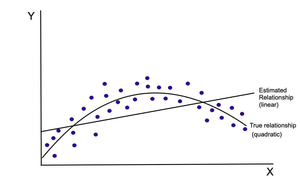
On the other hand, if the true relationship is the quadratic model appearing in equation 10.11, but a linear model is incorrectly selected, then an omitted variables problem occurs (since [latex]X_{i}^{2}[/latex] does not appear in the linear model). In this case, the intercept and slope estimators are biased (this case is illustrated in Figure 10.1).
The choice between a linear and a quadratic model is formally identical to determining whether an additional variable ([latex]X_{i}^{2}[/latex]) should be included in the regression equation. More generally, in the case of polynomial model specifications, an incorrect choice of functional form results in a regression equation that either includes variables that do not belong or excludes variables that belong in the equation. Thus, for polynomial model, the discussion of the two types of specification error above can be directly applied to the choice of functional form.
Selecting the functional form for a model also involves determining whether one or more dummy variables or interaction terms should be included.Suppose, for example, that an econometrician is trying to choose between the following two model specifications:
\begin{equation}Y_{i}=\beta _{0}+\beta _{1}X_{i}+\beta _{2}Z_{i}+u_{i}\tag{10.12}
\end{equation}
and
\begin{equation}
Y_{i}=\beta _{0}+\beta _{1}X_{i}+\beta _{2}Z_{i}+\beta _{3}(X_{i}Z_{i})+u_{i} \tag{10.13}
\end{equation}
In this case, the choice between equations 10.12 and 10.13 involves determining whether the interaction term [latex]X_{i}Z_{i}[/latex]) should be included in the regression equation. Omitting the interaction term when it belongs in the equation results in the possibility of biased and inconsistent parameter estimates; excluding a relevant interaction term from the regression results in inefficient parameter estimates.
10.1.4 Specification error in practice: bias vs. efficiency
In practice, an econometrician does not know the true relationship that exists between the dependent and independent variables. Instead, he or she must select the variables that are to be included in a regression equation. If relevant variables are left out of the equation, the estimated coefficients on the other variables will be biased and inconsistent. The inclusion of irrelevant variables results in inefficient, but unbiased and consistent, parameter estimates. Faced with this trade-off, most econometricians would argue that it is better to include too many rather than too few variables in the model.
Thus, when specifying an econometric model, a simple rule-of-thumb is that if you are not sure whether a particular variable belongs in the regression equation, it is safer to include it. If you find that a variable (or a set of variables) is not significant, then it is always possible to drop the variable in subsequent tests. By including an irrelevant variable, the worst thing that could occur is that the standard errors of the other estimators may be somewhat inflated. If the variable is omitted from an equation in which it belongs, all of the parameters (and [latex]t[/latex]-ratios) are subject to a potentially serious bias. When this occurs, it is quite possible that this bias may result in sign reversals in the estimated coefficients.
Since the choice of model specification is so important, a number of tests and procedures have been developed to aid in the process of model specification. Some of the more commonly used procedures are discussed below in section 10.5
10.2 Caution: Data mining
When conducting a research project, economists generally hope to find interesting (and statistically significant) results. This is as true for beginning students as it is for professional economists. Publication in professional journals is generally dependent upon the discovery (or confirmation) of interesting relationships among economic variables.
Students generally (mistakenly) believe that their research papers will receive higher grades if they can provide an equation with a high R[latex]^{2}[/latex] and high [latex]t[/latex]-ratios.
In order to achieve these “desirable” results, economists often estimate the parameters of a large number of alternative regression equations. These alternative model specifications are formed by adding and deleting variables in the equation and by experimenting with alternative functional forms. This process is known as data mining. High speed computers make it possible to quickly estimate a very large number of alternative model specifications. In fact, many statistical packages make it possible to automate this process to some extent.
Many econometricians view data mining as being unethical. The reason for this is somewhat obvious. Suppose that an econometrician estimates 100 alternative versions of an econometric model before finding a specification in which the sign of the “critical” variables are statistically significant and have the expected signs. If the econometrician only reports the results that appear to be the “best,” it is quite likely that these results are not indicative of the true relationship that exists among the variables. Hypothesis tests derived from models derived in such a manner should, at best, be treated with a high degree of caution.
It should be noted, however, that even ethical econometricians will often estimate more than one version of a model. Economic theory generally indicates what types of variables belong as independent variables in a regression model. This theory, however, does not usually dictate the precise functional form of the relationship, nor does it always specify the specific set of variables that belong in the equation. For example, economic theory predicts that the quantity of a good is inversely related to its own price. Theory also predicts that the demand for a good is affected by income and the prices of related goods and services. Economic theory, however, does not provide information about which particular goods are “related goods;” nor does it state whether the demand curve is best represented by a linear, log-linear, double-log, or polynomial relationship. In cases such as this, it is necessary to rely on empirical evidence to address these issues.
When a number of equations have been estimated in the process of formulating the final version of the equation, it is appropriate to describe the earlier estimates and the process by which the final model is selected. This allows readers to assess the appropriateness of the model selection procedure.
It should also be noted that it is inappropriate to rely on [latex]t[/latex]-ratios or [latex]F[/latex] statistics for hypothesis tests in the “final” version of a regression model if the choice of model specification was based, in part, on the magnitude of these statistics. If the variables included in a model were selected on the basis of their [latex]t[/latex]-ratios in a first-stage regression, then the distribution of the estimators in the second-stage regression is no longer a [latex]t[/latex]-distribution (since the second-stage hypothesis tests are not statistically independent of the first-stage tests). Thus, in interpreting regression results, it is important to recognize that the process of “data mining” results in the estimation of a final equation in which the estimated [latex]t[/latex]-ratios and [latex]F[/latex] statistics are inappropriate for hypothesis tests.
To see this problem, suppose that an econometrician considers 40 variables that might be included in a regression equation. Suppose that none of these variables have an effect on the dependent variable. If an equation is estimated in which all of these variables are included as regressors, it is expected that, on average, two of these variables would appear to be significant when a 5% significance level is chosen.[4] When the model is re-estimated using only the variables that appeared to be significant in the first-stage equation, it is quite likely that all of the variables in this new equation would appear to be significant, even though the true value of each coefficient is zero.
Since many reported studies are the result of some degree of “data mining,” it is always important to view new results with some skepticism. Most economists argue that a high degree of confidence can only be placed in results that are relatively “robust.” Results are said to be robust if similar results are found in numerous samples and under a variety of alternative model specifications.
10.3 Stepwise regression
One of the most commonly used tools for “data mining” is a stepwise regression procedure. Under a stepwise regression procedure, the researcher selects a set of independent variables that may belong as independent variables in a regression model. The statistical software package then uses a set of criteria to determine what variables to include in the regression equation. There are two basic types of stepwise regression procedures:
- a forward selection process in which the equation begins with a simple specification and adds variables to build a more complex model; and
- a backward selection process in which an elaborate model is specified and variables are eliminated in the process of forming the final model.
It should be noted that economists generally disapprove of stepwise regression procedures since the selection process is based upon statistical grounds rather than on theoretical grounds. Furthermore, as noted above, when the specification of the final version of a model is determined using [latex]t[/latex]-ratios or [latex]F[/latex] statistics, these statistics are not appropriate for use in hypothesis tests when the final model is estimated (since the second-stage test statistics are not statistically independent of those used in the first-stage model selection procedure). The stepwise regression procedure is discussed in this text because it is often used by practitioners (particularly in disciplines other than economics). The use of this procedure is not recommended.
10.3.1 Forward selection
When a stepwise regression model involves forward selection, the software package will first select the variable that is most highly correlated with the dependent variable and enter this variable as an independent variable in a bivariate regression model. If this variable is significant, the procedure will then find the variable that provides the largest incremental contribution to the regression equation and will add this variable to the regression. This process continues until a specified criterion (such as the maximization of the adjusted R[latex]^2[/latex]) is satisfied.
There is a very serious flaw with this methodological approach. Suppose the first stage equation is:
\begin{equation} Y_i=\beta _o+\beta _1X_i+u_i \tag{10.14} \end{equation}
This estimated equation serves as a basis to determine which of the remaining variable belong in the regression equation. If additional variables belong in this equation, however, the initial estimates of equation 10.14 are biased and inconsistent. At each stage of this procedure, the addition of new variables into the equation is determined through the use of estimates that are expected to be biased and inconsistent! Most econometricians find this approach somewhat troubling.
10.3.2 Backward selection
An alternative approach is to start with an equation that includes all variables that might belong in the equation and drop insignificant variables until some specified criterion is satisfied. The final equation involves one in which most (or all) of the variables remaining in the equation are statistically significant. A major problem with this procedure is that some variables that belong in the equation may be dropped if they are collinear with the remaining variables. If this occurs, the estimates of the remaining coefficients will be biased.
Many econometricians argue that a backward selection process is less troubling than a forward selection process. Econometricians, however, generally argue that model selection should be based, at least in part, on theoretical grounds. Thus, in reporting the results of econometric models, econometricians will generally include all variables that are theoretically relevant, even if some of the estimated coefficients are statistically insignificant.
Models selected on the basis of statistical correlations will always provide a good fit in the observed samples (since this is how the models are selected). If the model does not reflect causal relationships, however, the estimated model is not useful for hypothesis testing nor prediction purposes. (Recall the strong statistical relationship between mortality data and the number of secondary school teacher discussed in Chapter 1. Results of stepwise regression procedures should always be interpreted cautiously.
10.4 Model selection using adjusted R[latex]^{2}[/latex] and related criteria
While few econometricians use the stepwise regression procedure, it is not uncommon for econometricians to perform a search over several alternative model specifications. The adjusted R[latex]^{2}[/latex] provides a simple criteria that is often used to assist in model selection when economic theory does not provide guidance.[5] As noted above, however, criteria of this sort should be used only when economic theory does not provide predictions concerning the precise mix of variables that belong in an econometric model.
The same problems associated with the stepwise regression procedure described above, however, applies to the manual application of similar criteria in selecting alternative models. If it is inappropriate for a software package to automatically select independent variables in an attempt to maximize the adjusted R[latex]^{2}[/latex], it is just as inappropriate for an econometrician to do the same work manually.
Econometricians sometimes rely on adjusted R[latex]^{2}[/latex] (and similar criteria) to select among alternative models only when there is no theoretical reason to prefer one model specification over other specifications. It should be noted, though, that it is always inappropriate to use adjusted R[latex]^{2}[/latex] to compare alternative models in which different dependent variables are used in alternative models. Since this criteria relies on a comparison of the proportion of the variation in the dependent variable that is explained by variation in the independent variables, such a comparison only makes sense if the same dependent variable is used in each model. Thus, for example, a comparison of linear and double-log model specifications should never be based on a comparison of R[latex]^{2}[/latex] under the two model specifications. In general, however, even when a comparison of adjusted R[latex]^{2}[/latex] is possible, economists prefer to use more formal tests of model specification. The more commonly used test of model specification are discussed below.
10.5 Specification tests
Since the “true model” is not known by the researcher formulating a regression model, choices have to be made about which variables should be included in the equation. As noted above, this choice will be partly based on the predictions of economic theory. When theory generates ambiguous predictions, however, the choice must be made on empirical grounds. For example, while economic theory suggests that education and work experience should be included in an earnings equation, theory provides little evidence concerning what other demographic variables (such as gender, race, marital status, or geographical location) should be included in such an equation.
Suppose an econometrician wishes to investigate whether the variables [latex]X_{s+1}, X_{s+2},\ldots , X_k[/latex] should be added to (or dropped from) a regression model that already includes the variables [latex]X_1, X_2,\ldots, X_s[/latex]. A hypothesis test of this sort is referred to as a nested hypothesis test. In a nested hypothesis test, the variables in one version of the model are a subset of the variables included in the alternative model specification. A nonnested hypothesis test involves a choice between two regression equations in which neither equation consists of a set of variables that is a subset of the variables included in the other equation. In a nonnested hypothesis, each equation contains at least one independent variable that is not included in the other equation. Let’s first examine nested hypothesis tests. (Nonnested hypotheses are discussed in Section 10.7.)
10.5 Nested hypothesis tests
A nested hypothesis test in the multiple regression model involves a choice between two specifications:
\begin{equation*}\text{\textbf{Model\ I:}}\mathbf{\ }Y_{i}=\beta_{0}+\beta _{1}X_{1i}+\ldots +\beta _{s}X_{si}+u_{i},
\end{equation*}and\begin{equation*}
\text{\textbf{Model\ II:}}\mathbf{\ }Y_{i}=\beta_{0}+\beta _{1}X_{1i}+\ldots +\beta _{s}X_{si}+\beta _{(s+1)i}+\ldots +\beta _{k}X_{ki}+u_{i},
\end{equation*}
The choice between these two models is equivalent to a test of the null hypothesis:
\begin{equation}
\text{H}_{0}\text{: }\beta _{s+1}=\beta _{s+2}=\cdots =\beta _{k}=0 \tag{10.15}
\end{equation}
There are two commonly used methods for testing a null hypothesis of this sort: the Wald test (introduced in section 7.3.4) and the Lagrange multiplier test.[6]} Let’s examine these two test procedures.
10.6.1 The Wald test
As discussed in section 7.3.4, the Wald test involves the estimation of two models: an unrestricted model in which no restrictions are placed on the parameter values and a restricted model that imposes the restrictions appearing in the null hypothesis. An examination of Models I and II above indicates that Model I serves as the restricted model while Model II provides the unrestricted model. As in previous applications, the Wald test requires the construction of the statistic:
\begin{equation}
F=\frac{(\text{ESS}_{r}-\text{ ESS}_{u}\text{) }/\text{ }(m)}{\text{ESS}_{u} \text{ / [}N-(k+1)]} \tag{10.16}
\end{equation}
where:
- ESS[latex]_{r}[/latex] = error sum of squares in the restricted model
- ESS[latex]_{u}[/latex] = error sum of squares in the unrestricted model
- [latex]N[/latex] = number of observations
- [latex]k+1[/latex]= total number of parameters in unrestricted model
- [latex]m[/latex] = number of restrictions imposed ([latex]=k-s[/latex])
This statistic is distributed as an [latex]F[/latex] statistic with [latex]m[/latex] and [latex]N-(k+1)[/latex] degrees of freedom for the numerator and denominator terms, respectively. The null hypothesis above (10.15) should be rejected if and only if the value of this [latex]F[/latex] statistic exceeds the critical value for this distribution at the predetermined significance level.
If the null hypothesis cannot be rejected, then it may be appropriate to drop the variables [latex]X_{s+1},X_{s+2},X_k[/latex] from the regression model in subsequent experiments. As noted above, however, econometricians will often include these variables in any reported results if economic theory predicts that they belong in the model. In general, however, it is important to remember that econometricians use tests of this sort only when economic theory generates ambiguous predictions concerning whether the particular variables [latex]X_{s+1},X_{s+2},X_k[/latex] belong in the regression equation.
The Wald test is commonly used by econometricians who are attempting to determine whether a set of variables should be dropped from a regression model. Under this test, the investigator starts with the more elaborate model (Model II) and performs a test to determine whether some of the variables in this model should be dropped (to form Model I).
In some situations, however, an econometrician has specified a model and wishes to determine whether one or more other variables should be added to the model specification. Since this question essentially involves the choice between two models (such as Models I and II above), this issue can be investigated by the use of the Wald test. The Lagrange multiplier test, however, provides an alternative test that investigates the question of whether a set of variables should be added to a regression equation.
10.6.2 The Lagrange multiplier test
As in the case of the Wald test, the Lagrange multiplier test is used to help determine the choice between the two models:
\begin{equation}
\text{\textbf{Model\ I:}}\mathbf{\ }Y_{i}=\beta_{0}+\beta _{1}X_{1i}+\ldots +\beta _{s}X_{si}+u_{i}, \tag{10.17}
\end{equation}
and
\begin{equation}
\text{\textbf{Model\ II:}}\mathbf{\ }Y_{i}=\beta _{0}+\beta _{1}X_{1i}+\ldots +\beta _{s}X_{si}+\beta_{s+1}X_{(s+1)i}+\ldots +\beta _{k}X_{ki}+u_{i} \tag{10.18}
\end{equation}
Once again, choosing between these two models is equivalent to testing the null hypothesis:
\begin{equation}
\text{H}_{0}\text{: }\beta _{s+1}=\beta _{s+2}=\cdots =\beta_{k}=0 \tag{10.19}
\end{equation}
As noted above, the Wald test begins with the more elaborate specification (Model I) and attempts to determine whether it can be reduced to a simpler form (Model I). The Lagrange multiplier test reverses this process. Before examining the formal procedure for conducting this test, it might be helpful to first examine an overview of the test procedure.
The Lagrange multiplier test relies on a two-stage estimation procedure.footnote[7] In the first stage of this process, the parameters of the simpler specification (equation 10.17 ) are estimated using an OLS estimation procedure. The sample error terms from this first-stage regression represent that part of the variation in the dependent variable that cannot be explained by the variables [latex]X_{1}[/latex] through [latex]X_{s}[/latex]. In the second-stage of the Lagrange multiplier test, these sample residuals are regressed on the expanded set of independent variables ([latex]X_{1}, X_{2},\ldots,X_{k})[/latex]. If the simpler model is correct, this set of independent variables should have no significant effect on the sample residuals.[8] When the more elaborate specification (Model II) is correct, however, the additional variables [latex]X_{s+1}, X_{s+2},\ldots , X_{k}[/latex] will be able to explain some of the variation in the dependent variable that is not explained by the variables [latex]X_{1}, X_{2}\ldots , X_{k}[/latex].
Thus, a Lagrange multiplier test consists of the following steps:
Step 1: Estimate the parameters of the model that embodies the restrictions imposed under the null hypothesis (Model I) using an OLS estimation procedure. Use this estimated equation to generate sample residuals, [latex]\hat{u}_i[/latex], defined as:
\begin{equation}\hat{u}_i=Y_i-\hat{\beta}_o-\hat{\beta}_1X_{1i}-\cdots -\hat{\beta}_sX_{si} \tag{10.20}\end{equation} These residuals are a measure of the part of [latex]Y_i[/latex] that cannot be explained using a linear function of [latex]X_1,\ldots ,X_s[/latex].
Step 2: Regress the sample residuals against a constant term and all of the independent variables in the unrestricted version of the model (Model II):\begin{equation}\hat{u}_i=\gamma _o+\gamma _1X_{1i}+\ldots +\gamma _sX_{si}+\gamma _{s+1}X_{(s+1)i}+\ldots +\gamma _kX_{ki}+\epsilon _i \tag{10.21} \end{equation} Equation 10.21 is called an auxiliary regression.
Step 3: Use the results from the estimation of equation 10.21 to create the Lagrange multiplier statistic defined as:[9]\begin{equation*}\text{Lagrange multiplier statistic = }N\cdot \text{R}^{2} \end{equation*}
where:
- [latex]N[/latex] = number of observations}
- R[latex]^{2}[/latex] = the value of R[latex]^{2}[/latex] resulting from the estimation of equation 10.21.
Step 4: Reject the null hypothesis if the Lagrange multiplier statistic exceeds the critical value for a [latex]\chi ^2(k-s)[/latex] distribution at the predetermined significance level. If the null hypothesis can be rejected, then at least one of the coefficients associated with the additional variables is statistically significant. This suggests that Model II is a more appropriate specification than Model I.
To understand how the Lagrange multiplier test operates, an examination of the auxiliary regression model (equation 10.21 is in order. As a consequence of the OLS estimation procedure used to estimate the parameters of Model I, the sample residuals, [latex]\hat{u}_{i}[/latex], are independent of the variables [latex]X_{1i},X_{2i},\ldots ,X_{si}[/latex]. A regression against these variables alone would result in a value of R[latex]^{2}[/latex] equal to zero. Thus, a large R[latex]^{2}[/latex] for the auxiliary regression indicates that the additional variables [latex]X_{s+1},X_{s+2},\ldots ,X_{k}[/latex] are able to explain part of the variation in [latex]Y_{i}[/latex] that cannot be explained using only the variables contained in Model I.
10.6.3 Wald test vs. Lagrange multiplier test
As the size of the sample approaches infinity, the Wald test and the Lagrange multiplier tests are equivalent. In finite samples, however, these two tests may provide different outcomes.[10]To be safe, both tests should be used. When the two tests provide different conclusions, it is safest to select the more complex model (Model II) since the potential costs associated with including one or more irrelevant variables is generally perceived as being less severe than the cost of omitting a relevant variable.
In practice, the choice between using either the Wald test or the Lagrange multiplier test tends to be made on the basis of convenience. Note that the Wald test requires that the more complex model (the unrestricted model) be estimated, while the Lagrange multiplier test requires only the estimation of the simpler model (the restricted model). If, as in the example above, the choice is between two multiple regression models, both tests can be easily conducted (in fact, many econometric software packages have options that provide for the automatic execution of one or both of these test procedures). In other applications, however, the estimation of either the restricted or unrestricted models will be simpler than the estimation of the alternative model. Econometricians often use the Lagrange multiplier test in applications in which it is relatively more difficult to estimate the unrestricted model (since this procedure does not require the estimation of the unrestricted model).
10.6.4 Example: Earnings equation
Let’s consider the earnings equation discussed in Chapter 9.[11] Suppose an econometrician is trying to select between two models:
Model I:
\begin{equation}
\ln (\text{earnings}_{i})=\beta _{}+\beta _{1}\text{SC}_{i}+\beta _{2}\text{CD}_{i}+\beta _{3}\text{MA}_{i}+\beta _{4}\text{PhD}_{i} \tag{10.22}
\end{equation}\begin{equation*}
+\beta _{5}\text{Black}_{i}+\beta _{6}\text{Hispanic}_{i}+u_{i} \end{equation*}
Model II:
\begin{equation}\ln (\text{earnings}_{i})=\beta _{0}+\beta _{1}\text{SC}_{i}+\beta _{2}\text{CD}_{i}+\beta _{3}\text{MA}_{i}+\beta _{4}\text{PhD}_{i}
\tag{10.23}
\end{equation}
\begin{equation*}
+\beta _{5}\text{Black}_{i}+\beta _{6}\text{Hispanic}_{i}
\end{equation*}
\begin{equation*}
+\beta _{7}\text{experience}_{i}+\beta _{8}\left( \text{experience}_{i}\right) ^{2}+u_{i}
\end{equation*}
The choice between models I and II is equivalent to testing the null hypothesis:
H[latex]_0[/latex]: [latex]\beta _7=\beta _8=0[/latex]
In simple terms, the econometrician is trying to determine whether the work experience variables experience and experience[latex]^2[/latex] should be included in the regression equation. As noted above, this choice may be based upon either the Wald or Lagrange multiplier tests. Let’s examine each of these tests.
Wald test
To perform a Wald test, the following two equations were estimated:[12]} The data used to estimate the models below are contained in the file “nls72.dat.” (Note: the file contains observations on both males and females.)}
Restricted model (Model I):
\begin{equation}
\widehat{\ln (\text{earnings}_{i}\text{)}}=\underset{(532.42)}{10.00}+\underset{(1.80)}{0.057}\text{SC}_{i}+\underset{(8.26)}{0.24}\text{CD}_{i}+\underset{(5.31)}{0.22}\text{MA}_{i} \tag{10.24} \end{equation}
\begin{equation*}
+\underset{(9.06)}{0.48}\text{PhD}_{i}-\underset{(-4.09)}{0.19}\text{Black}_{i}-\underset{(-1.86)}{0.10}\text{Hispanic}_{i}
\end{equation*}
ESS[latex]_{r}[/latex] = 956.983
([latex]t[/latex]-statistics in parentheses)
Unrestricted model (Model II):
\begin{equation}
\widehat{\ln (\text{earnings}_{i})}=\underset{(190.92)}{9.37}+\underset{(2.45)}{0.073}\text{SC}_{i}+\underset{(8.50)}{0.23}\text{CD}_{i}+\underset{(7.01)}{0.28}\text{MA}_{i} \tag{10.25}
\end{equation}
\begin{equation*}
+\underset{(10.39)}{0.52}\text{PhD}_{i}-\underset{(-4.08)}{0.18}\text{Black}_{i}-\underset{(-1.50)}{0.077}\text{Hispanic}_{i}
\end{equation*}
\begin{equation*}
+\underset{(7.03)}{0.014}\text{experience}_{i}-\underset{(-3.04)}{0.000058} \left( \text{experience}_{i}\right) ^{2}
\end{equation*}
ESS[latex]_u[/latex]=862.089
\begin{equation*}
(t\text{-statistics in parentheses})
\end{equation*}
To test the null hypothesis, an $F$ statistic is calculated as: \begin{equation*}
F=\frac{(\text{ESS}_{r}-\text{ ESS}_{u}\text{) }/\text{ }(m)}{\text{ESS}_{u}\text{ / [}N-(k+1)]}
\end{equation*}
\begin{equation*}
=\frac{\left( 956.983-862.089\right) /2}{862.089/2724}
\end{equation*}
\begin{equation*}
=149.92
\end{equation*}
Since this value exceeds the critical value of an [latex]F[/latex] statistic at all conventional significance levels, the null hypothesis can be rejected. Thus, the Wald test indicates that Model II is the appropriate specification.
Lagrange multiplier test
To perform a Lagrange multiplier test, the parameters of Model I are estimated using an OLS estimation procedure. The estimated equation appears in equation 10.24 above. This equation is used to generate estimated residuals [latex]\hat{u}_{i}[/latex] that appear as the dependent variable in the regression equation:
\begin{equation}
\hat{u}_{i}=\beta_{0}+\beta _{1}\text{SC}_{i}+\beta _{2}\text{CD}_{i}+\beta _{3}\text{MA}_{i}+\beta _{4}\text{PhD}_{i}\tag{10.26}
\end{equation}
\begin{equation*}
+\beta _{5}\text{Black}_{i}+\beta _{6}\text{Hispanic}_{i}
\end{equation*}
\begin{equation*}
+\beta _{7}\text{experience}_{i}+\beta _{8}\left( \text{experience}_{i}\right) ^{2}+\epsilon _{i}
\end{equation*}
When the parameters of this equation are estimated by OLS, the following equation results:
\begin{equation}
\hat{u}_{i}=\underset{(12.60)}{-0.62}+\underset{(0.55)}{0.016}\text{SC}_{i}- \underset{(-0.19)}{0.0050}\text{CD}_{i}+\underset{(1.45)}{0.059}\text{MA}_{i}+\underset{(0.89)}{0.045}\text{PhD}_{i} \tag{10.27} \end{equation}
\begin{equation*}
+\underset{(0.23)}{0.010}\text{Black}_{i}+\underset{(0.45)}{0.023}\text{Hispanic}_{i}
\end{equation*}
\begin{equation*}
\underset{(7.03)}{0.014}\text{experience}_{i}-\underset{(-3.04)}{0.000058} \left( \text{experience}_{i}\right) ^{2}
\end{equation*}
R[latex]^{2}[/latex]=0.099
(t-statistics in parentheses)
The Lagrange multiplier test requires the use of the statistic: \begin{equation*}
\text{Lagrange multiplier statistic = }N\cdot \text{R}^{2} \end{equation*}
\begin{equation*}
=2733(0.099)=270.57
\end{equation*}
Under a 1% significance level, the critical value for a [latex]\chi ^{2}[/latex] statistic with 2 degrees of freedom is 9.21. Since the estimated Lagrange multiplier statistic exceeds this critical value, the null hypothesis should be rejected. Thus, the Lagrange multiplier test also indicates that Model II should be chosen over Model I.
10.7 Nonnested hypotheses
Nonnested hypothesis tests are used to compare alternative model specifications when neither model can be expressed as a subset of the other model. For example, consider the choice between the two models: \begin{equation*}
\text{\textbf{Model A:} }Y_i=\beta_0+\beta _1X_i+u_i\end{equation*}
and
\begin{equation*}
\text{\textbf{Model B:} }Y_i=\gamma _0+\gamma _1Z_i+v_i
\end{equation*}
The choice between models A and B involves a nonnested hypothesis test since neither model can be expressed as a subset of the other model.
The [latex]J[/latex]-test, developed by Davidson and MacKinnon (1981, 1982) is one of the most commonly used tests for selecting between the hypotheses: \begin{equation*}
\text{H}_{0}\text{: Model A is correct}
\end{equation*}
and
\begin{equation*}
\text{H}_{1}\text{: Model B is correct}
\end{equation*}
The [latex]J[/latex] test is conducted in the following manner:[13]
Step 1: Estimate the parameters of models A and B separately, and store the fitted values from these models as [latex]\widehat{QD_{i}^{A}}[/latex] and [latex]\widehat{\ln (QD)_{i}^{B}}.[/latex][14]
Step 2: Under the [latex]J[/latex] test procedure described above, the fitted values generated by one model are added as additional regressors in the estimation of the other model. In this variation of the [latex]J[/latex] test, however, Model A and Model B have different dependent variables. Thus, the predictions generated by each model must be transformed so that they are measured in the same manner as the dependent variable in the alternative model. The predicted value of quantity from Model A is converted into a predicted value of the natural log of quantity by creating a new variable equal to the natural log of QD_{i}^{A}:[15]
\begin{equation*}
\widehat{\ln (QD_{i}^{A})}=\ln (\widehat{QD_{i}^{A}}) \end{equation*}
where ([latex]\widehat{QD_{i}^{A}}[/latex]) is the predicted value of quantity demanded when Model A is estimated. The level of quantity demanded predicted by Model B can be computed as:\footnote{Here, use is made of the fact that the exponential and natural log functions are inverse functions. Thus,
[latex]e^{\ln (X)}=X[/latex]
It should also be noted that if model B is the correct model, [latex]\widehat{QD}_{i}^{B}[/latex] will be a biased, but consistent estimator of [latex]QD_{i}[/latex].
\begin{equation*}
\widehat{QD_{i}^{B}}=e^{\widehat{\ln (QD)_{i}^{B}}} \end{equation*}
where [latex]\widehat{\ln (QD_{i}^{B})}[/latex] is the predicted value of the dependent variable when model B is estimated.
Step 3: The following two equations are estimated: \begin{equation}
QD_{i}=\alpha _{o}+\alpha _{1}P_{i}+\alpha _{2}\left( \widehat{\ln (QD_{i}^{B})}-\widehat{\ln (QD_{i}^{A})}\right) +\epsilon _{i} \tag{10.34}
\end{equation}
and
\begin{equation}
\ln (QD)_{i}=\eta _{o}+\eta _{1}\ln (P_{i})+\eta _{2}(\widehat{QD_{i}^{A}}-\widehat{QD_{i}^{B}})+\epsilon _{i}^{\prime } \tag{10.35} \end{equation}
Step 4: Use the [latex]t[/latex]-statistics for the coefficients [latex]\alpha_{2}[/latex] and [latex]\eta _{2}[/latex] to compare the two models. As the sample size tends toward infinity, these [latex]t[/latex]-statistics are distributed as standard normal variates. If Model B is correct, then the coefficient [latex]\hat{\alpha}_{2}[/latex] should be statistically significant in equation 10.34 while [latex]\hat{\eta}_{2}[/latex] should be insignificant in equation 10.35. If Model A is correct, the coefficient [latex]\hat{\eta}_{2}[/latex] should be significant while the coefficient [latex]\hat{\alpha}_{2}[/latex] should be statistically insignificant.
10.8.3 Example: Student performance in a microeconomics class
Let’s consider an application of the [latex]P[/latex] test. Consider the following two specifications of a model explaining student performance on a microeconomics final exam:[16] \begin{equation*}
\text{Model A: \ Final}_{i}=\beta _{0}+\beta _{1}\text{SAT-V}_{i}+\beta _{2} \text{SAT-M}_{i}+\beta _{3}\text{HSGPA}_{i}+u_{i} \end{equation*}
and
\begin{equation*}
\text{Model B: \ ln(Final}_{i}\text{)}=\gamma _{0}+\gamma _{1}\ln (\text{SAT-V})_{i}+\gamma _{2}\ln (\text{SAT-M}_{i}\text{)}+\gamma _{3}\ln (\text{HSGPA}_{i}\text{)}+v_{i}
\end{equation*}
Note that there is no theoretical reason to prefer one of these model specifications over the other. It is reasonable to assume that past knowledge and academic performance, as measured by SAT scores and high school GPA affects performance in college courses, but there is no a priori reason to prefer a linear over a double-log specification for this relationship. Thus, it seems that the [latex]P[/latex] test may be appropriately applied to help select the functional form of this model.
When an OLS regression is performed on Model A, the following equation is estimated:[17]
\begin{equation}
\widehat{\text{Final}}_{i}^{A}=\underset{(-1.68)}{-35.366}+\underset{(2.02)}{0.029}\text{SAT-V}_{i}+\underset{(4.25)}{0.058}\text{SAT-M}_{i}+\underset{(1.74)}{0.372}\text{HSGPA}_{i} \tag{10.36} \end{equation}
([latex]t[/latex]-statistics in parentheses)
The estimated version of Model B is given by: \begin{equation}
\widehat{\ln (\text{Final}_{i}^{B}\text{)}}=\underset{(-2.68)}{-6.64}+\underset{(2.32)}{0.378}\ln (\text{SAT-V}_{i})+\underset{(4.47)}{0.795}\ln (\text{SAT-M}_{i}) \tag{10.37}
\end{equation}
\begin{equation*}
+\underset{(1.54)}{0.674}\ln (\text{HSGPA}_{i}) \end{equation*}
([latex]t[/latex]-statistics in parentheses)
To perform the [latex]P[/latex] test, the predicted values from equations 10.36 and 10.37 are used to construct the variables: \begin{equation*}
\widehat{\ln (\text{Final}_{i}^{B})}-\widehat{\ln (\text{Final}_{i}^{A})} \end{equation*}
and
\begin{equation*}
\widehat{\text{Final}}_{i}^{A}-\widehat{\text{Final}}_{i}^{B} \end{equation*}
When these variables are added as additional regressors in the appropriate equations, the following equations are estimated: \begin{equation*}
\widehat{\text{Final}}_{i}^{A}=\underset{(-1.66)}{-35.789}+\underset{(1.32)}{0.031}\text{SAT-V}_{i}+\underset{(4.10)}{0.058}\text{SAT-M}_{i}\underset{(1.46)}{+0.359}\text{HSGPA}_{i}
\end{equation*}
\begin{equation*}
-\underset{(-0.11)}{14.344}(\widehat{\ln (\text{Final}_{i}^{B})}-\widehat{\ln (\text{Final}_{i}^{A})})
\end{equation*}
and:
\begin{equation*}
\widehat{\ln (\text{Final}_{i}^{B}\text{)}}=\underset{(-2.68)}{-6.69}+\underset{(1.78)}{0.455}\ln (\text{SAT-V}_{i})+\underset{(4.46)}{0.797}\ln (\text{SAT-M}_{i})+\underset{(1.11)}{0.570}\ln (\text{HSGPA}_{i}) \end{equation*}
\begin{equation*}
+\underset{(0.39)}{0.029}(\widehat{\text{Final}}_{i}^{A}-\widehat{\text{Final}}_{i}^{B})
\end{equation*}
([latex]t[/latex]-statistics in parentheses)
Since the [latex]t[/latex]-statistics for the estimated coefficients on the generated variables are both insignificant at all conventional significance levels, the [latex]P[/latex] test is inconclusive. When this occurs, most researchers would select whichever model is more convenient for their purposes. In demand analyses, for example, a double-log specification might be selected since the estimated coefficients serve as measures of elasticities. For the case considered above, there is no compelling theoretical or empirical reason to prefer one specification over the other.
10.9 A general specification test: Ramsey’s RESET test
The tests and criteria described above are generally used to determine whether a specific variable (or set of variables) should be added to (or deleted from) a regression equation. Ramsey’s Regression Specification Error Test (or simply RESET) is a test to determine whether some form of specification error is present.F[18] Let’s examine this test.
Suppose the regression model is given by:
\begin{equation}
Y_i=\beta_0+\beta _1X_{1i}+\beta _2X_{2i}+\ldots +\beta _kX_{ki}+u_i \tag{10.38} \end{equation}
When the parameters of equation 10.38 are estimated using OLS, the sample regression function is:
\begin{equation} \tag{10.39}
\hat Y_i=\hat \beta _0+\hat \beta _1X_{1i}+\hat \beta _2X_{2i}+\ldots +\hat \beta _kX_{ki}
\end{equation}
To perform the RESET test, equation 10.39 is used to generate predicted values of [latex]\hat Y_i[/latex]as well as the squared ([latex]\hat Y_i^2[/latex]) and cubed ([latex]\hat Y_i^3[/latex]) values of this term. Using these terms, a new equation can be formulated as:
\begin{equation}
Y_i=\beta _0+\beta _1X_{1i}+\beta _2X_{2i}+\ldots +\beta _kX_{ki}+\gamma _1\hat Y_i^2+\gamma _2\hat Y_i^3+u_i
\tag{10.40} \end{equation}
The RESET test is performed by estimating the parameters of equation 10.40 and performing a test of the hypothesis:
H[latex]_{0}[/latex]: [latex]\gamma _{1}=\gamma _{2}=0[/latex]
Thus, a Wald test is used to determine whether the terms [latex]\hat{Y}_{i}^{2}[/latex] and [latex]\hat{Y}_{i}^{3}[/latex] have a joint effect on the level of [latex]Y_{i}[/latex]. To perform this test, it is necessary to compute the statistic: \begin{equation}
F=\frac{(\text{ESS}_{r}-\text{ ESS}_{u}\text{) / 2}}{\text{ESS}_{u}\text{ / [}N-(k+1)]} \tag{10.41}
\end{equation}
where ESS[latex]_{r}[/latex] is the residual sum of squares resulting from the estimation of equation 10.38 and ESS[latex]_{u}[/latex] is the residual sum of squares resulting from the estimation of equation 10.40. If this [latex]F[/latex] statistic exceeds the critical value at the selected significance level, then some form of misspecification is indicated. Note that the [latex]\hat{Y}_{i}^{2}[/latex] and [latex]\hat{Y}_{i}^{3}[/latex] terms should be insignificant if the original model provided an accurate representation of the data. If the addition of these terms significantly improves the explanatory power of the model, this may suggest that the independent variables contain some additional explanatory power that is not being adequately represented by the original model specification.
Ramsey has shown that a wide variety of specification error can be detected by the use of this test. Unfortunately, the RESET test provides no information about the type of specification error. If the RESET test indicates that specification error is present, then the investigator should carefully reconsider the model to investigate possible sources of specification error.[19]
10.9.1 Example: Student performance in a microeconomics class revisited
Let’s reconsider the linear specification of the model explaining student performance on a microeconomics final exam. The original model was given by:[20]
\begin{equation}
\widehat{\text{Final}}_{i}=\underset{(-1.68)}{-35.366}+\underset{(2.02)}{0.029}\text{SAT-V}_{i}+\underset{(4.25)}{0.058}\text{SAT-M}_{i}+\underset{(1.74)}{0.372}\text{HSGPA}_{i} \tag{10.42} \end{equation}
\begin{equation*}
\text{(}t\text{-statistics in parentheses)}
\end{equation*}
To test the adequacy of the specification used in equation 10.42 , Ramsey’s RESET test can be applied. Creating new variables defined as: \begin{equation*}
\widehat{\text{F2}}_{i}=\widehat{\text{Final}}_{i}^{2} \end{equation*}
and:
\begin{equation*}
\widehat{\text{F3}}_{i}=\widehat{\text{Final}}_{i}^{3}\text{,} \end{equation*}
the following equation is estimated:
\begin{equation}
\widehat{\text{Final}}_{i}=\underset{(-0.99)}{-768.33}+\underset{(1.00)}{0.45 }\text{SAT-V}_{i}+\underset{(1.00)}{0.91}\text{SAT-M}_{i}+\underset{(1.00)}{5.87}\text{HSGPA}_{i} \tag{} \end{equation}
\begin{equation*}
-\underset{(-0.91)}{0.342}\widehat{\text{F2}}_{i}+\underset{(0.88)}{0.003} \widehat{\text{F3}}_{i}
\end{equation*}
To perform the RESET test, a Wald test can be applied to test for the joint significance of the coefficients on the [latex]\widehat{\text{F2}}_{i}[/latex] and [latex]\widehat{\text{F3}}_{i}[/latex] variables. The [latex]F[/latex] statistic for this Wald test is: \begin{equation*}
F=\frac{(\text{ESS}_{r}-\text{ ESS}_{u}\text{) }/\text{ }m}{\text{ESS}_{u} \text{ / [}N-(k+1)]}
\end{equation*}
Since ESS[latex]_{r}[/latex](the error sum of squares in equation 10.42) equals 8779.1344 and ESS[latex]_{u}[/latex] (the error sum of squares in equation 10.43) equals 8683.0265, the [latex]F[/latex] statistic is: \begin{equation*}
F=\frac{(8779.1344-\text{ }8683.0265\text{) }/\text{ }2}{\text{8683.0265 / (99-6)}}
\end{equation*}
\begin{equation*}
=0.51
\end{equation*}
Under the null hypothesis, this statistic is distributed as an [latex]F[/latex] statistic with 2 and 93 degrees of freedom. Since this [latex]F[/latex] statistic is less than the critical value for this statistic at all conventional significance levels, the RESET test suggests that the original model provides an adequate representation of the data generating process.
10.10 Measurement error
Most economic variables are measured with some degree of error. Individuals often make errors in filling out survey responses. For example, when individuals are asked to supply their birth date on survey forms, an inordinate number will report that they were born on the day that the survey was conducted. Errors are also made in recording or tabulating raw data.
One interesting type of measurement error occurs when the theoretical variables are not observable. For example, econometricians can not directly observe an individual’s ability or expectations concerning future income or prices. In cases such as this, proxy variables are often used to capture the effect of the unobservable variable(s). Proxy variables are variables that are believed to be strongly correlated with the unobservable variable. For example, IQ or SAT scores are often used as proxy variables to represent an individual’s intellectual ability. Since an individual’s human capital cannot be observed, educational attainment and previous work experience are often used as proxy variables to capture the effect of human capital investments.
10.10.1 Error in measuring the dependent variable
Let’s examine the effect of errors that occur in measuring the dependent variable. Suppose the true value of the dependent variable is given by the variable [latex]Y_i[/latex]. The observed value of the dependent variable ([latex]Y_i^{*}[/latex]) is related to the true value by the relationship:
[latex]Y_i^{*}=Y_i+v_i[/latex]
where [latex]v_i[/latex]is the amount of measurement error in the dependent variable.
If the true relationship is given by:
\begin{equation}
Y_{i}=\beta _{0}+\beta _{1}X_{1i}+\beta _{2}X_{2i}+\ldots +\beta _{k}X_{ki}+u_{i} \tag{10.44}
\end{equation}
then the relationship between the observed value of $Y_{i}$ and the independent variables is given by:
\begin{equation}
Y_{i}^{\ast }=\beta _{0}+\beta _{1}X_{1i}+\beta _{2}X_{2i}+\ldots +\beta _{k}X_{ki}+u_{i}+v_{i} \tag{10.45}
\end{equation}
This equation may be simplified by defining a new error term, [latex]\epsilon_{i}[/latex], defined as:
\begin{equation*}
\epsilon_{i}=u_{i}+v_{i}
\end{equation*}
Using this definition, the observed relationship may be expressed as: \begin{equation}
Y_{i}^{\ast }=\beta _{0}+\beta _{1}X_{1i}+\beta _{2}X_{2i}+\ldots +\beta _{k}X_{ki}+\epsilon _{i} \tag{10.46} \end{equation}
It is generally assumed that the measurement error ([latex]v_{i}[/latex]) is independent of the independent variables and the error term [latex]u_{i}[/latex].[21]} It is also typically assumed that the measurement error is just as likely to result in overstating as understating the value of the dependent variable. In other words, it is assumed that:[22]
[latex]E(v_{i})=0[/latex]
Under these conditions, the presence of measurement error in the dependent variable simply increases the variance of the error process.[23]
As long as all of the other conditions of the classical regression model are satisfied, the OLS estimators of the parameters in equation 10.46 are still unbiased. In fact, OLS estimators of the parameters of this equation are still best linear unbiased estimators (BLUE). There is, however, a cost associated with the presence of measurement error. Since the variance of the error term is greater when the dependent variable is measured with error, the standard errors of the parameter estimates will be greater than they would be if the true value of the dependent variable ([latex]Y_{i}[/latex]) had been observed. The existence of measurement error also lowers the R[latex]^{2}[/latex]for the equation (by increasing the sum of squared residuals).
10.10.2 Error in measuring an independent variable
The situation is somewhat more serious, however, when one of the independent variables is measured with error. Suppose that the relationship between the dependent variable and the true value of the independent variable is given by:
\begin{equation}
Y_i=\beta _0+\beta _1X_i+u_i \tag{10.47} \end{equation}
If the independent variable is measured with error, the relationship between the observed value of the independent variable ([latex]X_i^{*}[/latex]) and the true value ([latex]X_i[/latex]) is given by:
\begin{equation}
X_i^{*}=X_i+v_i \tag{10.48}
\end{equation}
It is generally assumed that the error term in this relationship ([latex]v_i[/latex]) has a mean of zero and is independent of [latex]u_i[/latex] and [latex]X_i[/latex].
Using the definition in equation 10.48, the relationship between the dependent variable and the observed values of the independent variable can be expressed as:
\begin{equation}
Y_i=\beta _0+\beta _1(X_i^{*}-v_i)+u_i \tag{10.49}
\end{equation}
or:
\begin{equation*}
Y_i=\beta _0+\beta _1X_i^{*}-\beta _1v_i+u_i \end{equation*}
Defining a new residual term, [latex]\epsilon_i[/latex] as: \begin{equation*}
\epsilon _i=u_i-\beta _1v_i
\end{equation*}
equation 10.49 may be restated as: \begin{equation*}
Y_i=\beta_0+\beta _1X_i^{*}+\epsilon _i
\end{equation*}
Unfortunately, the observed value of the independent variable [latex]X_{i}^{\ast }[/latex] and [latex]\epsilon_{i}[/latex] are correlated in this model. This can be demonstrated fairly easily by using the definitions for [latex]X_{i}^{\ast }[/latex] and [latex]\epsilon_{i}[/latex] :
\begin{equation*}
cov(X_{i}^{\ast },\epsilon _{i})=cov(X_{i}+v_{i},u_{i}-\beta _{1}v_{i}) \end{equation*}
\begin{equation*}
=E\left[ (X_{i}+v_{i}-\mu _{X})(u_{i}-\beta _{1}v_{i})\right] \end{equation*}
\begin{equation*}
=X_{i}E(u_{i})+E(v_{i}u_{i})-\mu _{X}E(u_{i})-\beta _{1}X_{i}E(v_{i})-\beta _{1}E(v_{i}^{2})+\beta _{1}\mu_{X}E(v_{i})
\end{equation*}
\begin{equation*}
=-\beta _{1}E(v_{i}^{2})
\end{equation*}
\begin{equation*}
=-\beta _{1}var(v_{i})\neq 0
\end{equation*}
This correlation between the error term and independent variable violates one of the conditions of the classical regression model. When the error terms are correlated with one or more independent variables, the OLS estimators of the intercept and slope terms are biased and inconsistent.[24]
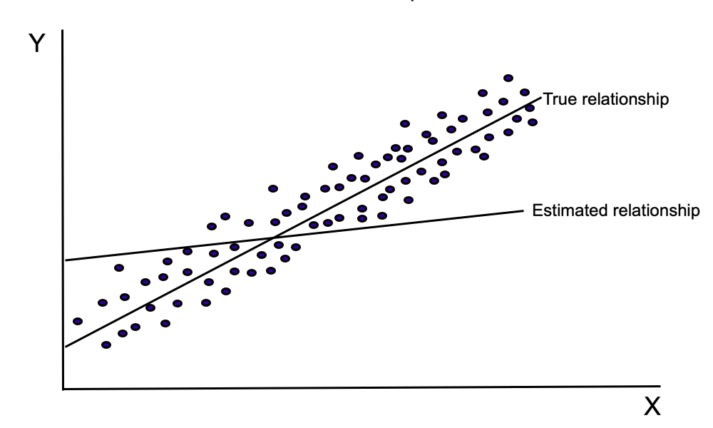
Figure 10.2 illustrates the effect of measurement error on parameter estimation. Since there is a negative covariance between [latex]X_{i}^{\ast }[/latex] and [latex]\epsilon _{i}[/latex], the error terms become progressively smaller as [latex]X_{i}[/latex] increases. As this diagram illustrates, positive errors are more likely to occur when the level of [latex]X[/latex] is low while negative errors are more likely to occur when the level of [latex]X[/latex] is high. When an OLS estimation procedure is used to estimate the parameters of this equation, the estimated slope and intercept terms are biased.
Measurement error in survey data
Anyone who has examined actual responses to survey data will often be dismayed by the number of inconsistent responses on some of the forms. For example, individuals who claim to be physicians will sometimes report that they have not completed high school. Quite often, these mistakes involve someone inadvertently listing a wrong code or filling in the wrong circle on a survey form.
In some cases, however, individuals may systematically provide incorrect responses. Grubb (1993), for example, compares actual educational attainment with self-reported levels of educational attainment for participants in the National Longitudinal Stdy of the High School Class of 1972. In this study, Grubb finds that individuals with low levels of measured ability and low high school grades tend to overstate their level of educational attainment. Individuals with high levels of measured ability, however, tend to provide accurate measures of educational attainment. This result suggests that estimates of the rate of return to higher education based on self-reported data may understate the actual return to education (since some low ability individuals who have not attended college are inappropriately classified as college attendees).
10.10.3 Instrumental variables estimator
A relatively simple procedure is available to correct for the presence of measurement error. This procedure relies on the use of an instrumental variables estimator. An instrumental variables estimator relies on a two-stage estimation procedure in which a least-squares regression is performed in each stage.[25] Let’s consider the simple model discussed above: \begin{equation}
Y_i=\beta_0+\beta _1X_i^{*}+\epsilon _i \tag{10.50} \end{equation}
where [latex]X_i^{*}[/latex] is the observed value of [latex]X_i[/latex]. As before, the observed value ([latex]X_i^{*}[/latex]) differs from the true value ([latex]X_i)[/latex] as a result of measurement error. To correct for this problem:
Step 1: Find one or more variables that are both correlated with [latex]X_i[/latex] and uncorrelated with the residual. These variables are known as instrumental variables. For simplicity, let’s assume that variable [latex]Z_i[/latex] satisfies these requirements.
Step 2: Use an OLS estimation procedure to estimate the parameters of the regression equation:
\begin{equation}
X_i^{*}=\gamma _0+\gamma _1Z_i+w_i \tag{10.51} \end{equation}
(where [latex]w_i[/latex] is a random error term that is uncorrelated with the measurement error). This is the first-stage regression.
Step 3: Use the estimated parameters from this first-stage to generate predicted values of [latex]X_i^{*}[/latex] using the formula: \begin{equation}
\hat{X}_i^{*}=\hat{\gamma}_o+\hat{\gamma}_1Z_i \tag{10.52} \end{equation}
Many econometric software packages provide simple commands that automatically generate the predicted values from a regression procedure.
Step 4: In equation 10.50, replace the observed values of the independent variable with the predicted values given in equation 10.52 to form the equation:
\begin{equation}
Y_{i}=\beta _{0}+\beta _{1}\hat{X}_{i}^{\ast }+\epsilon _{i} \tag{10.53}
\end{equation}
Estimate the parameters of this equation using an OLS estimation procedure.
In this second-stage regression, the correlation between [latex]\hat{X}_{i}^{\ast }[/latex] and the error term [latex]\epsilon_{i}[/latex] will approach zero as the sample size increases since [latex]\hat{X}_{i}^{\ast }[/latex] is a linear function of [latex]Z_{i}[/latex] (which is independent of [latex]\epsilon _{i}[/latex]). The estimated values of the intercept and slope parameters in this second-stage regression equation provide consistent estimates of the corresponding population parameters.[26]
Before attempting to implement this procedure manually, you may wish to check to see if your software package provides a instrumental variables estimator. Most econometric software packages contain routines that automate this process.[27]
10.10.4 Example: Measurement error in earning equations
An interesting example of the use of an instrumental variables estimator to correct for a measurement error problem is provided by Griliches and Mason (1972) in their study of the effects of education and ability on earnings. As Griliches and Mason note, econometricians do not directly observe the ability of individuals. Instead, the researcher, at best, observes the individuals’ scores on standardized exams. While these test scores serve as a measure of the individual’s ability, this measure is not a perfect measure of the individual’s ability. Therefore, the use of test scores in place of the individual’s actual ability serves as an example of a measurement error problem. The ability variable used by Griliches and Mason in their study was the individual’s score on the Armed Forces Qualifications Test (AFQT).
They assume that this test serves as an unbiased measure of an individual’s true ability. Since this test score, however, may either overstate or understate the individual’s true ability, a measurement error problem occurs. To correct for this, Griliches and Mason used an instrumental variables estimator in which a set of family background and predetermined variables (such as parents’ social class, the individual’s geographical location during adolescence, and the level of education acquired prior to entering the military) serve as instruments for the test score variable. It is argued that these variables are correlated with the individual’s ability, but are uncorrelated with the error term in the earnings equation (thereby satisfying the two conditions required of instrumental variables).
To investigate the effect of measurement error on parameter estimates, Griliches and Mason estimated several alternative earnings equations using both an OLS and an IV estimation procedure. Table 10.1 contains the estimated parameters (and standard errors) for one of the models estimated in their study.[28]
| Variable Name | [latex]\underset{\text{(s.e. in parentheses)}}{\text{OLS Estimates}}[/latex] | [latex]\underset{\text{(s.e. in parentheses)}}{\text{IV Estimates}}[/latex] |
|---|---|---|
| Race[latex]_i[/latex] | [latex]\underset{(0.0458)}{0.1982}[/latex] | [latex]\underset{(0.0468)}{0.0730}[/latex] |
| Schooling[latex]_i[/latex] | [latex]\underset{(0.0067)}{0.0331}[/latex] | [latex]\underset{(0.0065)}{0.00483}[/latex] |
| AFQT[latex]_i[/latex] | [latex]\underset{(0.00038)}{0.00298}[/latex] | |
| [latex]\widehat{\text{AFQT}}_{i}[/latex] | [latex]\underset{(0.00078)}{0.00889}[/latex] |
where:
- Race[latex]_{i}[/latex] = 1 if person i is white
- Schooling[latex]_{i}[/latex] = years of schooling acquired during or after military service
- AFQT[latex]_{i}[/latex] = Armed Forces Qualifications Test
The estimates appearing in Table 10.1` indicate that a correction for measurement error results in a fairly large effect on the magnitude of the estimated coefficients. In particular, the instrumental variables estimates suggests that the OLS estimates overstates the effect of race and understates the effect of ability.
Proxy variables
Many economic variables are not directly observable. For example, econometricians cannot directly observe an individual’s “ability” or his or her expectations about future prices and income. When unobservable variables play an important role in an economic model, econometricians often attempt to use proxy variables to represent the effect of these variables. The use of proxy variables is a special case of the measurement error problem discussed above. The proxy variable is essentially equivalent to an inaccurately measured independent variable.
While an instrumental variables estimator makes it possible to correct for a measurement error problem associated with the use of proxy variables, these techniques are not generally applied in practice. The primary reason for this is that the correction procedure requires the discovery of instruments that are both uncorrelated with the error term and highly correlated with the variable(s) that are measured with error. These new variables, of course, must be free of measurement error. In practice, the discovery of such variables is often problematic. For this reason, applied econometricians generally will report the possible presence of measurement error, but generally do not apply this corrective technique unless it is believed that the problem is particularly severe.
Consider, for example, the instrumental variables used by Griliches and Mason. As Taubman (1972) notes, it is quite possible that the demographic and family background variables used as instruments for the ability variable are correlated with unobservable factors that influence individual earnings. If, for example, the earnings of the respondents are directly affected by the socioeconomic status of their parents, then one of the instruments will be correlated with the errors in the earning equations. In this case, the IV estimation procedure will generate biased and inconsistent parameter estimates (since the fitted values will still be correlated with the error terms).
Thus, when proxy variables are used in place of an unobservable independent variable, the resulting parameter estimates are biased and inconsistent. Unfortunately, however, there is no good alternative to their use. Since the underlying variable cannot be observed, omitting the proxy variable(s) from the equation will also result in biased and inconsistent estimates (due to an omitted variable bias). Under these circumstances, econometricians generally have tended to introduce proxy variables to capture the effect of the unobservable variables that are theoretically important in the relationship. It is generally believed that it is better to attempt to control for theoretically important factors and risk the associated measurement error problem than to omit an important variable and face an omitted variable bias.[29]
Summary
In this chapter, a number of problems dealing with model specification have been discussed. The issue of specification error is one that every econometrician must deal with in specifying an econometric model. There is a cost associated with any form of misspecification. Biased and inconsistent parameter estimates may occur if a relevant variable is excluded from the regression equation. An efficiency loss occurs when irrelevant variables are included in the equation.
The choice among alternative functional forms should be guided by economic theory whenever possible. Previous studies may also offer some suggestions concerning an appropriate functional form. When economic theory and past research do not offer useful indications, the choice among alternative functional forms may be guided by the use of Wald tests, Lagrange multiplier tests, [latex]J[/latex] tests, [latex]P[/latex] tests, or the RESET test.
If the dependent variable in a regression model is subject to measurement error, the variance of the estimators increases, but the estimators remain unbiased (as long as the measurement error is uncorrelated with the independent variables). Measurement error occurring in one or more of the independent variables, however, results in biased and inconsistent parameter estimates. The use of proxy variables to capture the effect of unobservable variables provides a common situation in which measurement error occurs. An instrumental variables, estimator, however, may be used to provide consistent parameter estimates when one or more of the independent variables are measured with error.
Key Concepts
- specification error
- omitted variable bias
- data mining
- stepwise regression
- nested hypothesis test
- nonnested hypothesis test
- Wald test
- Lagrange multiplier test
- auxiliary regressions
- [latex]J[/latex] test
- [latex]P[/latex] test
- RESET test
- measurement error
- instrumental variables estimator
- instruments
- proxy variables
Exercises and problems
- Suppose that the actual population earnings equation is given by: \begin{equation*}
\text{Earnings}_{i}=\beta _{0}+\beta _{1}\text{Experience}_{i}\text{ + } \beta _{2}\text{Schooling}_{i}+u_{i}\end{equation*}
where:
- Earnings[latex]_{i}[/latex] = annual earnings of individual [latex]i[/latex]
- Experience[latex]_{i}[/latex] = years of work experience for person [latex]i[/latex]
- Schooling_{i} = years of education for person [latex]i[/latex]
- [latex]\beta _{1}>0[/latex], and[latex]\beta _{2}>0[/latex].
An econometrician, however, incorrectly estimates a model given by:
\begin{equation}
\text{Earnings}_{i}=\gamma_{0}+ \gamma _{1}\text{Schooling}_{i}+u_{i} \tag{10.54}
\end{equation}
Use equation 10.6 to determine the conditions under which the OLS estimator [latex]\hat{\gamma}_{1}[/latex] is a biased estimator of [latex]\beta _{2}[/latex].
\item Suppose that the parameters of equation 10.54 are estimated using a random sample of the population. Is it likely that the OLS estimator [latex]\hat{\gamma}_{1}[/latex] will be a biased estimator of [latex]\beta_{2}[/latex]?
Will [latex]\hat{\gamma}_{1}[/latex] be expected to overstate or understate the parameter [latex]\beta_{2}[/latex]? Explain.
\item Use equation 10.6to explain the circumstances under which the bias associated with an omitted relevant variable will be positive? When will the bias be negative?
\item Which type of specification error is more serious: excluding a relevant variable or including an irrelevant variable? Explain your response.
\item Suppose that the true value of the constant term [latex]\beta _{0}[/latex] is zero in the equation:
\begin{equation*}
Y_{i}=\beta _{0}+\beta _{1}X_{1i}+\beta _{2}X_{2i}+u_{i} \end{equation*}
What are the consequences of estimating the model using an equation in which a constant term is present?
Since [latex]\beta _{0}=0[/latex] is there any advantage to estimating the parameters of the following equation?
\begin{equation*}
Y_{i}=\beta _{1}X_{1i}+\beta _{2}X_{2i}+u_{i} \end{equation*}
\item Compare the estimated coefficients and [latex]t[/latex]-ratios on the variables experience and experience[latex]^{2}[/latex] in equations 10.25 and 10.27. Provide an intuitive explanation for this result.
\item In Section 10.6.4, both the Wald and the Lagrange multiplier tests suggested that the experience[latex]_{i}[/latex] and experience[latex]_{i}^{2}[/latex] terms should remain in the regression equation. Suppose, however, that one or both of these tests suggested that these variables were not statistically significant. Should an econometrician exclude these variables in future estimates of earnings equations? Explain.
\item Use the estimated parameters and $t$-ratios from equation 10.25 to determine whether the effect of work experience on log-earnings is best represented by a linear or a quadratic relationship.
(Perform the appropriate test at a 1% significance level).
\item In their empirical analysis of faculty salaries, Haignere, Lin, Eisenberg, and McCarthy (1996, p. 54) argue that the choice between a linear and quadratic model should be determined by the following criteria: “You can examine this by noting the amount of improvement in the R[latex]^{2}[/latex] when the quadratic term is entered. If there is no sizable increase in the R[latex]^{2}[/latex], then the analysis does not need the quadratic term.”
\item Would an econometrician agree with this statement? Why or why not?
\item What alternative procedures might be used by an econometrician to perform such a specification test?
\item In their empirical analysis of faculty salaries, Haignere, Lin, Eisenberg, and McCarthy (1996, p. 65) suggest that it is preferable to use “salary” rather than ln(salary) as the dependent variable in an earnings equation: “Our preference for Salary rather than Logged Salary as the dependent variable is based on simplicity and the logic of studying what people actually take home in their paychecks.”
\item Is this an appropriate rationale for selecting between these functional forms? Why or why not?
\item Could a specification test help to resolve this issue? If so, which test(s)?
\item Consider the two regression models given by: \begin{equation*}
\text{Model I: Earnings}_{i}=\beta _{0}+\beta _{1}\text{AFQT}_{i}+\beta _{2} \text{WW}_{i}+\beta _{3}\text{Female}_{i}
\end{equation*}
\begin{equation*}
+\beta _{4}\text{Health}_{i}+\beta _{5}\text{Black}_{i}+\beta _{6}\text{Hisp} _{i}+\beta _{7}\text{Asian}_{i}
\end{equation*}
\begin{equation*}
+\beta _{8}\text{NatAmer}_{i}+\beta _{9}\text{NE}_{i}+\beta _{10}\text{NortCent}_{i}
\end{equation*}
\begin{equation*}
+\beta _{11}\text{South}_{i}+\beta _{12}\text{Rural}_{i}+\beta _{13}\text{YearEd}_{i}+u_{i}
\end{equation*}
and:
\begin{equation*}
\text{Model II: Earnings}_{i}=\gamma _{0}+\gamma _{1}\text{AFQT}_{i}+\gamma _{2}\text{WW}_{i}+\gamma _{3}\text{Female}_{i} \end{equation*}
\begin{equation*}
+\gamma _{4}\text{Health}_{i}+\gamma _{5}\text{Black}_{i}+\gamma _{6}\text{Hisp}_{i}+\gamma _{7}\text{Asian}_{i}
\end{equation*}
\begin{equation*}
+\gamma _{8}\text{NatAmer}_{i}+\gamma _{9}\text{Rural}_{i}+\beta _{10}\text{YearEd}_{i}+v_{i}
\end{equation*}
(Definitions of these variables appear in question 24 in Chapter 9.)
\item Use the data in the file “nlsy.dat” to estimate the parameters of each of these models.
\item Perform a Wald test to compare these two model specifications.
\item Perform a Lagrange multiplier test to compare these two model specifications.
\item Do these tests agree?
\item Use the data in the file “nlsy.dat” to perform a RESET test of Model I in question 24. What does this test suggest?
\item Consider the following two models describing the 1992 Presidential election:
\begin{equation}
\text{Model I: DVOTE}_{i}=\beta _{0}+\beta _{1}\text{UN}_{i}+\beta _{2}\text{FEDFUNDS}_{i} \tag{10.55}
\end{equation}
\begin{equation*}
+\beta _{3}\text{DEFENSE}_{i}+\beta _{4}\text{CRIME}_{i} \end{equation*}
\begin{equation*}
+\beta _{5}\text{NE}_{i}+\beta _{6}\text{S}_{i}+\beta _{7}\text{W}_{i}+u_{i} \end{equation*}
and
\begin{equation}
\text{Model II: DVOTE}_{i}=\gamma _{0}+\gamma _{1}\text{UN}_{i}+\gamma _{2} \text{FEDFUNDS}_{i} \tag{10.56} \end{equation}
\begin{equation*}
+\gamma _{3}\text{DEFENSE}_{i}+\gamma _{4}\text{CRIME}_{i}+v_{i} \end{equation*}
\item Use the data contained in the file “election.dat” to estimate the parameters of each of the above models.
\item Perform a Wald test to compare these two model specifications.
\item Perform a Lagrange multiplier test to compare these two model specifications.
\item Do these tests agree?
\item Use the data contained in the file “election.dat” to estimate the parameters of equations 10.55 and 10.56.
\item Perform a RESET test on each of these equations. What do these tests suggest?
\item A simple form of Milton Friedman’s permanent income hypothesis is given by the following consumption function model: \begin{equation*}
\text{C}_{t}=\beta _{0}+\beta _{1}\text{YP}_{t}+u_{t} \end{equation*}
where:
- C[latex]_{t}[/latex] = consumption spending
- YP[latex]_{t}[/latex] = permanent income
Permanent income, however, is not observed. Instead, we observe current disposable personal income (YD[latex]_{t}[/latex]). Disposable personal income at time [latex]t[/latex] equals the sum of permanent income and a random component, [latex]v_{t}[/latex]. In mathematical terms:
\begin{equation*}
\text{YD}_{t}=\text{YP}_{t}+v_{t}
\end{equation*}
\item Express the relationship that exists between C[latex]_{t}[/latex] and YD[latex]_{t}[/latex].
\item Suppose an equation is estimated of the form: \begin{equation*}
\text{C}_{t}=\alpha _{0}+\alpha _{1}\text{YD}_{t}+\epsilon _{t} \end{equation*}
Will the estimated parameters [latex]\hat{\alpha}_{0}[/latex] and [latex]\hat{\alpha}_{1}[/latex] serve as unbiased estimators of \beta _{0} and [latex]\beta _{1}[/latex]? Why or why not?
\item Could an instrumental variables estimator be used here? What is required for a variable to serve as an instrumental variable in this model?
\item The [latex]J[/latex] test performed in Section 10.8.1 was performed using a sample consisting solely of males. Perform the same test using a sample of females using the data contained in the file “nls72.dat.” (Note: since this data set contains both males and females, only female observations should be selected for the estimation process.) Does a similar result occur for females?
\item Use the data in the file “final.dat” to verify the reported [latex]P[/latex] test results appearing in section 10.8.3.
\item Use a [latex]P[/latex] test to determine whether a linear or a Cobb-Douglas production function best captures the relationship between output and labor and capital inputs in the service sector. Use the data contained in the file “service.dat” to perform this analysis. What does this test suggest?
\item Suppose that you are asked to formulate an equation that explained student GPAs as a function of the students’ ability and demographic characteristics. Since student ability cannot be directly measured, it is decided that you will rely on SAT scores as a proxy for student ability.
\item How will the use of a proxy variable of this sort affect the estimated coefficients?
\item Would it be better to omit this variable from the equation?
\item An econometrician specifies a regression model as: \begin{equation*}
Y_{i}=\beta _{0}+\beta _{1}X_{1i}+\beta _{2}X_{2i}+u_{i} \end{equation*}
In this equation, the variable [latex]X_{2i}[/latex] is a measure of individual income.
She discovers that this variable is recorded using the midpoints of relatively large intervals so that the observed level of income for each individual contains some amount of measurement error.
\item What problem(s) would be associated with direct OLS estimation of this equation?
\item Carefully describe how an instrumental variables estimator can be used to remedy this problem.
\section{Mathematical Appendix}
\subsection{Specification error: omitted variable bias} In the model discussed in section 10.1.2, the true model is: \begin{equation} \tag{10.57}
Y_i=\beta _0+\beta _1X_i+\beta _2Z_i+u_i \end{equation}
but an econometrician mistakenly specifies the model as: \begin{equation} \tag{10.58}
Y_i=\gamma _0+\gamma _1X_i+v_i
\end{equation}
Equation 10.57 implies that: \begin{equation*}
\sum Y_{i}=N\beta _{0}+\beta _{1}\sum X_{i}+\beta _{2}\sum Z_{i}+\sum u_{i} \end{equation*}
Multiplying both sides of this equation by 1/N, this becomes: \begin{equation*}
\frac{1}{N}\sum Y_{i}=\beta _{0}+\beta _{1}\frac{1}{N}\sum X_{i}+\beta _{2} \frac{1}{N}\sum Z_{i}+\frac{1}{N}\sum u_{i} \end{equation*}
or:
\begin{equation}
\overline{Y}=\beta _{o}+\beta _{1}\overline{X}+\beta _{2}\overline{Z}+\overline{u} \tag{10.59}
\end{equation}
Subtracting equation 10.59 from equation 10.57 results in: \begin{equation*}
Y_{i}-\overline{Y}=\beta _{1}\left( X_{i}-\overline{X}\right) +\beta _{2}\left( Z_{i}-\overline{Z}\right) +\left( u_{i}-\overline{u}\right) \end{equation*}
Thus, the estimated value of [latex]\gamma[/latex] equals: \begin{equation*}
\hat{\gamma}_{1}=\frac{\sum \left( X_{i}-\overline{X}\right) \left[ \beta _{1}\left( X_{i}-\overline{X}\right) +\beta _{2}\left( Z_{i}-\overline{Z} \right) +\left( u_{i}-\overline{u}\right) \right] }{\sum \left( X_{i}- \overline{X}\right) ^{2}}
\end{equation*}
\begin{equation*}
=\frac{\beta _{1}\sum \left( X_{i}-\overline{X}\right) ^{2}}{\sum \left( X_{i}-\overline{X}\right) ^{2}}+\frac{\beta _{2}\sum \left( X_{i}-\overline{X}\right) \left( Z_{i}-\overline{Z}\right) }{\sum \left( X_{i}-\overline{X} \right) ^{2}}+\frac{\sum \left( X_{i}-\overline{X}\right) \left( u_{i}- \overline{u}\right) }{\sum \left( X_{i}-\overline{X}\right) ^{2}} \end{equation*}
\begin{equation*}
=\beta _{1}+\beta _{2}\frac{\sum \left( X_{i}-\overline{X}\right) \left( Z_{i}-\overline{Z}\right) }{\sum \left( X_{i}-\overline{X}\right) ^{2}}+ \frac{\sum \left( X_{i}-\overline{X}\right) \left( u_{i}-\overline{u}\right) }{\sum \left( X_{i}-\overline{X}\right) ^{2}} \end{equation*}
The expected value of the estimated parameter [latex]\hat{\gamma}[/latex] equals: \begin{equation*}
E\left( \hat{\gamma}\right) =E\left( \beta _{1}\right) +\beta _{2}E\left( \frac{\sum \left( X_{i}-\overline{X}\right) \left( Z_{i}-\overline{Z}\right) }{\sum \left( X_{i}-\overline{X}\right) ^{2}}\right) +E\left( \frac{\sum \left( X_{i}-\overline{X}\right) \left( u_{i}-\overline{u}\right) }{\sum \left( X_{i}-\overline{X}\right) ^{2}}\right) \end{equation*}
Since the [latex]X[/latex]‘s and [latex]Z[/latex]‘s are assumed to be constant, the expected value of the second term is simply the term itself. The expected value of the last term equals zero because [latex]X_{i}[/latex] and [latex]u_{i}[/latex] are independent by assumption.
Thus, the expected value of the slope estimator in the incorrectly specified equation is:
\begin{equation*}
E\left( \hat{\gamma}\right) =\beta _{1}+\beta _{2}\left( \frac{\sum \left( X_{i}-\overline{X}\right) \left( Z_{i}-\overline{Z}\right) }{\sum \left( X_{i}-\overline{X}\right) ^{2}}\right) \end{equation*}
Thus, it can be easily seen that the estimated slope parameter ([latex]\hat{\gamma}[/latex]) is biased. The amount of the bias equals: \begin{equation}
\text{bias(}\hat{\gamma}\text{) = }\beta _{2}\left( \frac{\sum \left( X_{i}- \overline{X}\right) \left( Z_{i}-\overline{Z}\right) }{\sum \left( X_{i}- \overline{X}\right) ^{2}}\right) \tag{10.61} \end{equation}
The first term in this product equals the slope coefficient on the omitted variable. The second term is equal to the estimated slope coefficient, $\hat{% \alpha}_{1}$ in the regression equation: \begin{equation*}
Z_{i}=\alpha _{o}+\alpha _{1}X_{i}+\epsilon _{i} \end{equation*}
With a little bit of algebraic manipulation, equation 10.60 can be restated as:
\begin{equation}
\text{bias(}\hat{\gamma}\text{) = }\beta _{2}\left( \frac{\left( \frac{1}{N-1 }\right) \sum \left( X_{i}-\overline{X}\right) \left( Z_{i}-\overline{Z} \right) }{\left( \frac{1}{N-1}\right) \sum \left( X_{i}-\overline{X}\right) ^{2}}\right) \tag{10.60} \end{equation}
The numerator in the ratio on the right-hand side of equation 10.61 equals the sample covariance between [latex]X_{i}[/latex] and [latex]Z_{i}[/latex] while the denominator is the sample variance of [latex]X_{i}[/latex]. Thus, the bias can be compactly expressed as:
\begin{equation*}
\text{bias(}\hat{\gamma}\text{) = }\beta _{2}\left( \frac{\hat{\sigma}_{XZ}}{\hat{\sigma}_{X}^{2}}\right)
\end{equation*}
Using this result, the expected value of the slope parameter [latex]\hat{\gamma}[/latex] can be restated as:
\begin{equation*}
E\left( \hat{\gamma}\right) =\beta _{1}+\beta _{2}\left( \frac{\hat{\sigma} _{XZ}}{\hat{\sigma}_{X}^{2}}\right)
\end{equation*}
- Some econometricians use the term specification error more broadly to include choices among alternative functional forms. The effect of using an improper functional form is, in some cases, equivalent to the problem of either excluding a relevant variable or including an irrelevant variable. This possibility is discussed in subsection 10.1.3 A more general discussion of the choice among alternative functional forms appears in sections 10.5 -10.8. ↵
- A proof of this proposition appears in the mathematical appendix at the end of this chapter. ↵
- The interested reader may find a proof in a more advanced text. See, for example, the discussion in Greene (2000), pp. 334-7. ↵
- Remember that when a 5% significance level is chosen, a variable that does not belong in the equation will appear to be significant 5% of the time. ↵
- In addition to the use of adjusted R[latex]^{2}[/latex], a number of other criteria have been devised to help select the mix of variables that should be included in a regression model. A discussion of a wide variety of such criteria appears in Ramanathan (1998), pp. 164-6. Most modern econometric packages automatically provide estimates for one or more of these criteria (in addition to the adjusted R[latex]^{2}[/latex]). ↵
- A third form of test, known as a ``likelihood-ratio test'' is also sometimes used for tests of this sort. A brief discussion of the use of likelihood-ratio tests appears in Chapter 14. In practice, however, the Wald and Lagrange multiplier test are the most commonly used tests in a regression framework. A good comparison of these tests appears in Engle (1984). ↵
- This version of the Lagrange multiplier test is based upon the work of Engle (1982). A more complete discussion of the Lagrange multiplier test requires mathematical tools beyond the scope of this text. Readers familiar with matrix algebra and multivariate calculus may find a more complete discussion in Silvey (1959), Buse (1982) or Engle (1982). ↵
- Remember, these sample residuals represent only that part of the variation that has not already been explained by the variables [latex]X_{1}[/latex] through [latex]X_{s}[/latex] . If the additional variables do not explain any of the variation in [latex]Y_{i}[/latex] (after controlling for the effect of the variables [latex]X_{1}, X_{2},\ldots , X_{k}[/latex]), then they should not be able to account for any variation in the sample residuals. ↵
- In large samples, this statistic is approximately distributed as a [latex]\chi ^{2}[/latex] statistic with [latex]k-s[/latex] degrees of freedom. ↵
- When used to test for the joint significance of a set of variables in a multiple regression model, the Lagrange multiplier statistic provides a somewhat more stringent standard for rejecting the null hypothesis. Thus, it is possible that the null hypothesis may be rejected under the Wald test but not rejected under the Lagrange multiplier test. If the null hypothesis is rejected under the Lagrange multiplier test, however, it will always be rejected under the Wald test. A good discussion of this argument appears in Maddala (1992), pp. 120-4. ↵
- A description of these variables appears in Table 9.3 in Chapter 9. ↵
- These equations are estimated using a sample consisting of 2733 males who were participants in the National Longitudinal Study of the High School Class of 1972. ↵
- Strictly speaking, this test is only valid in large samples. In practice, however, it is often used in small samples as well. ↵
- Most econometric software packages contain an option that allows you to automatically save the predicted values when a regression equation is estimated. ↵
- It should be noted that if model A is the correct model, [latex]ln(\widehat{QD}_{i}^{A})[/latex] will be a biased, but consistent estimator of [latex]ln(QD_{i})[/latex]. (This is a biased estimator because, as noted in earlier chapters, [latex]E(g(X))[/latex] will not, in general, be equal to [latex]g(E(X))[/latex].) ↵
- The linear form of this model was first discussed in In Chapter 6. ↵
- The data used for this estimation appears in the file ``final.dat.'' This data set consists of 99 observations on student performance on a final exam in an introductory microeconomics class, their SAT verbal and math scores, and their high school GPA. ↵
- or a more complete description of this test, see Ramsey (1969). ↵
- If this test indicates that a form of misspecification is present, this may be the result of heteroskedasticity, autocorrelation, or simultaneous equation problems. These topics are discussed in later chapters. ↵
- This model was first discussed in Chapter 6. The data used for this estimation appears in the file ``final.dat.'' ↵
- If the measurement error, [latex]v_{i}[/latex], is correlated with any of the independent variables, then biased and inconsistent parameter estimates will result. In practice, economists generally assume that the error in measuring the dependent variable is not related to the level of any of the independent variables. If the measurement error is due to random recording errors or imprecise measurement of the dependent variable, this is probably a safe assumption. There are cases, though, where this independence assumption is inappropriate. Suppose, for example, that an earnings equation is estimated and individuals with low levels of educational attainment are more likely to overstate their income than individuals with higher levels of education. In this case, estimates of the rate of return to education would be subject to a downward bias (since the average increase in earnings associated with a higher level of education is understated). ↵
- A biased estimate of the intercept term will occur if this assumption is violated. The estimators for the slope coefficient remain unbiased (as long as all of the other conditions of the classical regression model are satisfied). Thus, a nonzero expectation for [latex]v_{i} [/latex]will not alter the outcome of hypothesis tests involving only the slope parameters. ↵
- The variance of [latex]\epsilon_{i}[/latex] is given by: \begin{equation*}var(\epsilon_{i})=var(u_{i})+var(v_{i})\end{equation*} since [latex]u_{i} [/latex]and [latex]v_{i}[/latex] are assumed to be independent. ↵
- A proof of this result requires mathematical tools beyond the scope of this text. An interested reader may find a proof in Greene (2000), pp. 375-80. ↵
- Another application of this instrumental variables estimator occurs in the estimation of simultaneous equation systems. The instrumental variables estimator discussed in this chapter is equivalent to the two-stage least squares (2SLS) estimator that will be discussed in Chapter 15. While these estimators are equivalent, the term ``two-stage least squares'' is often reserved for the application of this estimator to models involving simultaneous equations. Because these two estimators are equivalent, however, econometric software packages may refer to this estimator as either an IV estimator or a 2SLS estimator. ↵
- It should be noted that the instrumental variables estimator is biased in finite samples because a nonzero correlation still exists between [latex]\hat{X}_{i}^{\ast } [/latex]and [latex]\epsilon _{i}[/latex] (since [latex]\hat{\gamma}_{0}[/latex] and [latex]\hat{\gamma} _{1}[/latex] are not independent of [latex]\epsilon _{i}[/latex] in the first stage regression). ↵
- This is especially desirable since the standard errors appearing in the second-stage OLS regression are not consistent. A relatively simple adjustment is required when a ``generated'' regressor of this sort is included in the regression equation. This adjustment is provided by the 2SLS procedures available on all major econometrics packages. A full discussion of this adjustment requires mathematical tools beyond the scope of this text. A good simplified discussion appears in Maddala (1992), pp. 374-376. ↵
- While other variable (such as age, work experience, current geographical location, and length of active military service) are included in these equations, the estimated coefficients and standard errors are not presented in this paper. ↵
- McCallum (1972) and Wickens (1972) have shown that a greater degree of inconsistency occurs when such proxy variables are omitted from the equation. Aigner (1974), on the other hand, notes that when the precision of the estimators is taken into account, the result is less straightforward. ↵
