test
8.5 Marginal effects and elasticities
In the preceding sections of this chapter, it was shown that OLS estimation techniques can be applied to the estimation of a variety of functional forms. Once these equations have been estimated, however, it is often useful to measure the magnitude of the effect resulting from a change in an independent variable. For example, when a market researcher estimates a demand equation, it is important to know the magnitude of the change in quantity demanded that results from a change in price or income. To measure the magnitude of effects such as this, economists generally rely on two alternative measures:
- marginal effects, and
- elasticities.
The marginal effect associated with a change in an independent variable is, roughly speaking, the change in the dependent variable that occurs when there is a one-unit change in the level of an independent variable.[1]
\begin{equation*}\text{marginal effect of }X_{j}\text{ on }Y\text{ = }\frac{\Delta Y}{\Delta X_{j}}\end{equation*}
holding constant the level of all other independent variables.
| Model | Equation | Marginal Effect | Elasticity |
|---|---|---|---|
| Reciprocal | [latex]Y_i=\beta_0+\beta_1\frac{1}{X_i}[/latex] | [latex]-\beta_1/X^2[/latex] | [latex]-\beta_1/XY[/latex] |
| Log-Log | [latex]ln(Y)=ln(\beta_0)+\beta_1ln(X)[/latex] | [latex]\beta_1Y/X[/latex] | [latex]\beta_1[/latex] |
| Linear log | [latex]Y=\beta_0+\beta_1ln(X)[/latex] | [latex]\beta_1/X[/latex] | [latex]\beta_1/Y[/latex] |
| Log-linear | [latex]ln(Y)=\beta_0+\beta_1X[/latex] | [latex]\beta_1Y[/latex] | [latex]\beta_1X[/latex] |
| Linear | [latex]Y=\beta_0+\beta_1X[/latex] | [latex]\beta_1[/latex] | [latex]\beta_1X/Y[/latex] |
| Quadratic | [latex]Y=\beta_o+\beta_1X+\beta_2X^2[/latex] | [latex]\beta_1+2\beta_2X[/latex] | [latex]\frac{(\beta_1+2\beta_2X)X)}{Y}[/latex] |
| Cubic | [latex]Y=\beta_0+\beta_1X+\beta_2X^2+\beta_3X^3[/latex] | [latex]\beta_1+2\beta_2X+3\beta_3X^2[/latex] | [latex]\frac{(\beta_1+2\beta_2X+3\beta_3X^2)X)}{Y}[/latex] |
In many cases, however, economists wish to measure the magnitude of an effect using a measure of elasticity. As noted in section 8.4.1, the elasticity of [latex]Y[/latex]with respect to[latex]X_{j}[/latex] is a measure of the percentage change in [latex]Y[/latex] that results from a one-percent change in the level of [latex]X_{j}[/latex]. In mathematical terms, this elasticity can be expressed as:
elasticity of [latex]Y[/latex] with respect to [latex]X_{j}[/latex] =[latex]\frac{\%\Delta \text{ in }Y}{\%\Delta \text{ in }X_{j}}[/latex]
When estimating demand functions, for example, economists are often interested in estimating the price elasticity of demand, the cross-price elasticity of demand, and the income elasticity of demand.
The Price Elasticity of Demand for Marijuana
Nisbet and Vakil (1972) attempted to measure the price elasticity of demand for marijuana among UCLA students. Using data from an anonymous survey (conducted by mail), they estimated both linear and double-log demand specifications. Using actual purchase data, the estimated equations were:
\begin{equation*}\widehat{\text{Qm}_i }= 3.236 – 0.225\text{Pm}_i – 0.002 \text{E}_i +0.036 \text{S}_i\end{equation*}
\begin{equation*}\widehat{ln(\text{Qm})} = 2.609 – 01.013 ln(\text{Pm}_i) – 0.311 ln(\text{E}_i) +0.404 ln(\text{S}_i)\end{equation*}
where:
- Qm[latex]_i[/latex] = quantity of marijuana purchased per month (in ounces)
- Pm[latex]_i[/latex] = price of marijuana (in dollars)
- E[latex]_i[/latex] = a measure of mean monthly expenditure
- S[latex]_i[/latex] = a measure of expenditure dispersion
In this sample, the average price of marijuana was $10 per ounce and the average quantity purchased was 1.49 ounces per month. As Table 8.1 indicates, under the linear specification, the price elasticity of demand (evaluated at the sample mean price and quantity) equals:
[latex]\hat{\beta}_{1}\left( \frac{\overline{Pm}}{\overline{Qm}} \right) = -0.225 \left( \frac{10.0}{1.49} \right) = -1.51[/latex]
Under the double-log specification, the estimated price elasticity of demand is simply equal to 1.013, the estimated coefficient on the log of the price variable.
As noted in Chapter 6, when a model is linear in variables the slope coefficients, [latex]\beta _{j}[/latex], serve as a measure of the marginal effect associated with a one-unit change in [latex]X_{j}[/latex], holding constant all of the other independent variables. Under the reciprocal, log, and polynomial models considered above, however, the marginal effect associated with a change in the level of an independent variable cannot be as simply measured. As noted above, the estimated intercept and slope parameters are measures of elasticities under the double-log specification. Under alternative model specifications, however, elasticities vary with the level of the dependent and/or independent variables. Table 8.1 provides a listing of the marginal effects and elasticities associated with a change in an independent variable under alternative model specifications.
An examination of Table 8.1 indicates that the marginal effect or elasticity associated with a particular independent variable may be a function of the level of either the dependent or the independent variable. When this occurs, economists often report the value of the marginal effects (or elasticities) measured at particular values of the dependent and independent variables.
In cross-sectional or longitudinal studies, the marginal effects (or elasticities) are generally reported for a “representative” observation. This generally means that the marginal effects are evaluated by setting the values of the independent variable(s) and the dependent variable to their sample means. In time-series analyses, however, economists are generally more interested in recent outcomes. Thus, marginal effects may be evaluated by setting the values of the dependent and independent variables equal to the most recently observed values.
A superficial examination of Table 8.1 may suggest that the use of the linear regression model is most appropriate when an economist is interested in estimating marginal effects, while the log-log specification should be used to estimate elasticities. Unfortunately, however, the simplest approach is not always the most appropriate approach. The choice among alternative functional forms should be based on the nature of the relationship that exists between the dependent variable and the set of independent variables. If it is believed that the marginal effect is constant for all levels of an independent variable, then a linear specification is most appropriate. If, however, it is believed that the magnitude of the marginal effect varies with the level of the independent variable, then an alternative functional form should be used that more closely approximates the economic process that generates the data.
8.6 Selecting a functional form
It should be noted that a regression model will often include more than one of the transformations described above. For example, it is quite possible that a regression model may be specified as:
[latex]Y_{i}=\beta _{o}+\beta _{1}\frac{1}{X_{i}}+\beta _{2}\ln (Z_{i})+\beta_{3}S_{i}+\beta _{4}S_{i}^{2}+u_{i}[/latex]
or:
[latex]\ln (Y_{i})=\beta_{0}+\beta_{1}X_{i}+\beta_{2}X_{i}^{2}+\beta_{3}Z_{i}+u_{i}[/latex]
In selecting the specific form of a regression relationship, an econometrician should take into account the nature of the relationship that exists between the dependent and independent variables. For example, the unemployment rate can never be less than 0% nor greater than 100%. If the unemployment rate is specified as either a dependent or independent variable, this characteristic should be taken into account (as in the reciprocal relationship discussed above). The earnings equation discussed below provides another case where economic theory provides some evidence that can be used to help select a model specification.
One strategy that is often used by practicing econometricians is to examine the model specifications used in previous studies of the same (or a closely related) topic. If previous researchers make a compelling case for a particular specification, then that specification often provides a useful starting point for future research. Of course, one should never accept an inappropriate model specification solely because it has been used before.
Quite often, however, the appropriate specification of an econometric model cannot be determined a priori. Prior studies may either not exist or may provide a variety of alternative model specifications. Under these circumstances, the choice of model specification is generally based upon empirical criteria.[2] An examination of appropriate empirical methods of selecting among alternative model specifications is the focus of Chapter 10.
For now, it can be noted economists sometimes select among alternative models by comparing the R[latex]^{2}[/latex] (or [latex]\overline{\mathrm{R}}^2[/latex]).of these models. While this approach is commonly used, a few qualifications should be made:
- Economists prefer to use economic theory to determine model specification. Those variables that are included in economic models because they are of theoretical importance should not be dropped from equations simply because this leads to a higher value of R[latex]^{2}[/latex] (or [latex]\overline{\mathrm{R}}^2[/latex]). R[latex]^{2}[/latex] is a measure of statistical association, and is not a measure of causation. Models based on causal relationships are expected to generate better predictions than models based on correlations that may be spurious.
- Since R[latex]^{2}[/latex] (or [latex]\overline{\mathrm{R}}^2[/latex]) provides a measure of the proportion of the variation in the dependent variable that is accounted for by the regression equation, it may be used to compare alternative models in which the dependent variable is the same. It is always inappropriate to use R[latex]^{2}[/latex] (or [latex]\overline{\mathrm{R}}^2[/latex]) as a criteria to select among competing models when the dependent variable differs across these models. For example, R[latex]^{2}[/latex] does not provide a meaningful comparison between linear and double-log models.
8.6.1 Example: An estimated earnings equation
The estimation of earnings equations has kept hundreds of econometricians busy for much of the past 25 years. By estimating variations of equation 8.29}, econometricians have been able to investigate such issues as: the rate of return to education, male-female wage differentials, racial wage differentials, and a wide variety of other issues. Let’s examine a simple earnings equation.
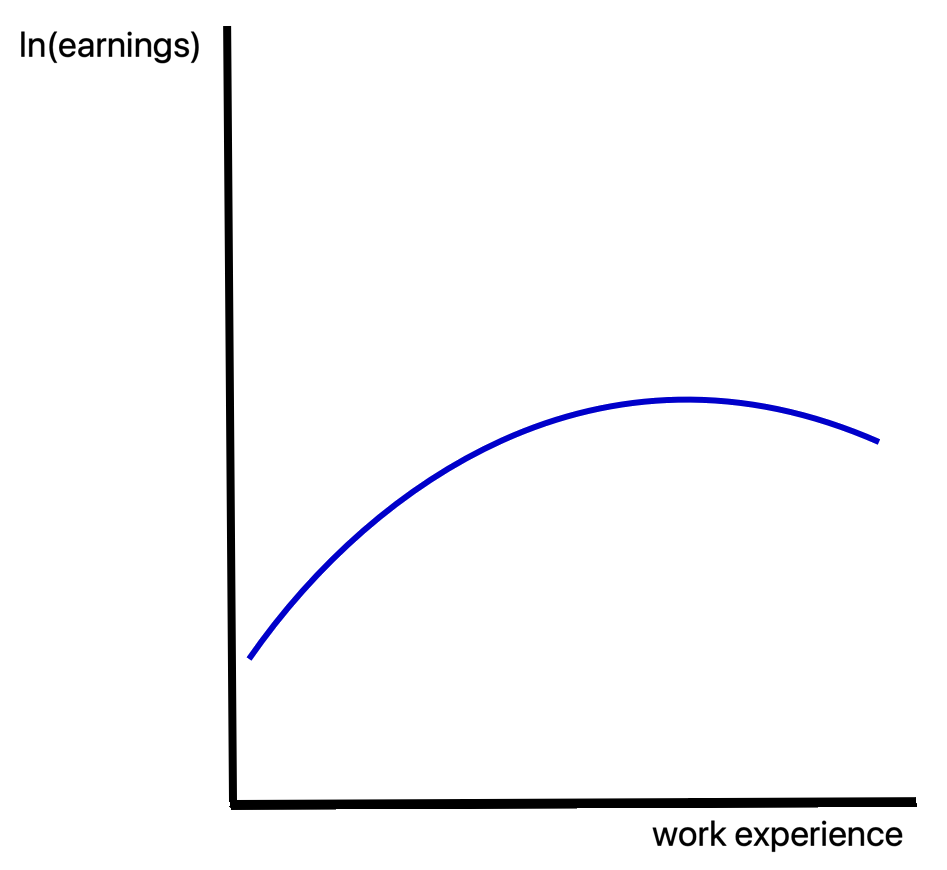
A large amount of theoretical work and empirical evidence indicates that earnings increase with work experience.[3] Earnings increase, however, by progressively smaller increments with each additional year of experience. Human capital theory provides a relatively simple explanation for this phenomena. The return to investments in education, health care, and on-the-job training are larger when the investment occurs at a relatively young age (since the benefits are realized over a longer time period). Thus, human capital investments tend to decline with age. Since human capital depreciates over time (as training becomes obsolete and skills deteriorate), earnings increase more rapidly during early stages of an individual’s career. As the individual ages, earnings will either increase more slowly, or may even decrease. Figure 8.8 illustrates the relationship between log earnings and work experience.
The discussion above suggests that an appropriate specification for an earnings equation is:
[latex]\ln(\mathrm{earnings}_i)=\beta_{0}+\beta_{1}\mathrm{experience}_i+\beta_{2}\mathrm{experience}^{2}+u_i \tag{8.31}[/latex]
where:
- earnings[latex]_{i}[/latex] = respondent’s earnings in 1985 (in 1985 dollars)
- experience[latex]_{i}[/latex] = months of work experience at the respondent’s two most recent jobs
This specification involves a combination of the log-linear and polynomial transformations. When the parameters of equation 8.31 are estimated using a sample of 3992 males that were participants in the National Longitudinal Study of the High School Class of 1972,[4]the estimated equation is:
\begin{equation}\widehat{\ln (\text{earnings}_{i})}=\underset{(236.95)}{9.377}+\underset{(10.676)}{0.01734}\text{experience}_{i}-\underset{(-5.780)}{0.0000904}\text{experience}_{i}^{2} \tag{8.32}\end{equation}
([latex]t[/latex]-ratios in parentheses)
Each of the estimated coefficients in equation 8.32 are significantly different than zero at all conventional significance levels. Notice that the estimated coefficient [latex]\hat{\beta}_{2}[/latex] is relatively small compared to the value of [latex]\hat{\beta}_{1}[/latex].[5] This combination of a positive value for [latex]\hat{\beta}_{1}[/latex] and a negative value (that is smaller in magnitude) for [latex]\hat{\beta}_{2}[/latex] is consistent with the inverted U-shaped earnings profile appearing in Figure 8.8.A[6]
Since equations of this sort are often used to investigate the rate of return to education, let’s examine how the results appearing in equation 8.32 may be used for this purpose. Under this relatively standard specification, the percentage increase in earnings resulting from an additional year of education is given by:[7]
[latex]\%\Delta[/latex] in earnings[latex]_{i}[/latex] = ([latex](\beta _{1}+2\beta_{2})[/latex]experience[latex]_{i}\times 100\%[/latex]
Using the estimates appearing in equation 8.33, each additional month of work experience increases earnings by:
[latex]\%\Delta[/latex] in earnings[latex]_{i}[/latex]= [latex](0.01734-0.0001808) \times[/latex] experience[latex]_{i}) \times 100\% \tag{8.33}[/latex]
This equation suggests that the first month of work experience will, on average, cause earnings to increase by:
[latex](0.01734-0.0001808(1)) \times 100\% = 1.72\%[/latex]
An inspection of equation 8.33, however, indicates, that the percentage increase in earnings becomes progressively smaller as the level of work experience increases. For example, the 30th month of work experience will result in an average increase in earnings by:
[latex](0.01734-0.0001808(30)) \times 100\%=1.19\%[/latex]
In fact, this equation suggests that earnings will begin to decline for individuals who have received more than 96 months of work experience. This equation suggests that the 97th month of work experience results in a 0.02% decline in earnings. Is this result likely?
The simple answer to this is: “probably not.” The earnings equation estimated above is unlikely to provide very reliable information about the effect of additional work experience on earnings. It is likely that the earnings equation specified in equation 8.31 does not contain all of the variables that affect an individual’s earnings. In particular, individuals with higher levels of educational attainment tend to earn more. Since all of the individuals in this sample are approximately the same age, those with more education also tend to have less work experience. The relatively high rate of return to work experience for those with less work experience is likely to be partly due to the higher educational attainment of these individuals.[8] As will be shown more formally in Chapter 10, the omission of variables that belong in a regression model can result in biased estimates of model parameters.
In practice, most empirical studies do find that earnings decline beyond some level of work experience. In general, however, these studies tend to suggest that the decline in earnings occurs at a much higher level of work experience than is found using the relatively simple model discussed above. Thus, the specific estimates discussed above should not be taken too seriously. The method used to estimate the percentage increase in earnings resulting from an additional unit of work experience, however, can be applied whenever the dependent variable is the log of earnings and the independent variables include both an “experience” and an “experience[latex]^{2}[/latex]” term. While earnings equations tend to include a variety of additional right-hand side variables, virtually all of them use this basic specification.
In Chapter 9, we will examine a more elaborate earnings equation that takes work experience, education, and other variables into account.
8.7 Summary
In this chapter, it has been shown that the linear regression model can be applied to a wide variety of models after a suitable transformation of variables. The most commonly used transformations are the polynomial, reciprocal, and log transformations. These transformations substantially expand the range of models that can be estimated through linear regression techniques.
By carefully analyzing the process that generates the observed data, it is often possible to specify a functional form that provides a close approximation to the underlying relationship. When economic theory and knowledge of institutional processes does not provide such guidance, other criteria must be adopted to select an appropriate functional form. In simple bivariate relationships, plotting the data will often provide some guidance. Under the more general case of multiple regression analysis, however, a variety of empirical tests exist that may be used to guide specification choices. Tests of this sort will be discussed in Chapter 10.
The marginal effects and elasticities resulting from a change in an independent variable have also been addressed in this chapter. It was noted that, under most model specifications, the marginal effects and elasticities are functions of the level of the dependent variable, the independent variable, or both. The marginal effect is constant for all values of the dependent and independent variables only in the linear model. Elasticities are constant for all values of the dependent and independent variables only in the double-log model.
8.8 Key Concepts
- linearity
- linear in parameters
- linear in variables
- reciprocal transformation
- log transformation
- double-log models
- semi-log models
- linear-log models
- log-linear models]
- polynomial transformations
- marginal effects
- elasticity
- More precisely, when the dependent variable ([latex]Y[/latex]) is a function of a single independent variable ([latex]X[/latex]), the marginal effect is measured by the derivative ([latex]\frac{dY}{dX}[/latex]). If a multiple regression model, the marginal effect of a change in the [latex]j[/latex]th independent variable is measured by the partial derivative ([latex]\frac{\partial Y}{\partial X_{j}}[/latex]). ↵
- In the special case of a bivariate relationship, an examination of a scatterplot of the dependent and independent variables will often suggest an appropriate specification. Scatterplots, however, are not very useful for this purpose in a multiple regression framework. Even in the case of bivariate regression relationships, though, model specifications based on observed data, rather than on an appropriate model of the underlying causal relationships, may lead to results that are misleading, and nongeneralizable to other samples. ↵
- The theoretical basis of age-earnings profiles is discussed in Becker (1993). Most current studies of the empirical relationship between age and earnings are based on the seminal work of Mincer (1974). ↵
- All members of this particular sample are full-time workers. The work experience variable is defined as the total number of months spent working at the worker's two most-recent jobs (including the present job). Most studies, however, use a different measure of work experience that is based upon the number of years worked. In particular, many econometricians have followed Mincer (1974) in defining work experience as age minus years of schooling. The data used to generate the results reported below is a subsample drawn from the National Longitudinal Study of the High School Class of 1972. In this data set, the only measure of recent work experience is a series of questions that ask the respondent for the starting and ending dates for their most recent jobs. This information has been used to generate the measure of recent work experience used in this equation. The data used in this estimation can be found in the file ``exp1.dat.'' ↵
- One of the reasons for the difference in the magnitude of the coefficients in this equation is the rather large difference in the magnitude of these variables. In the early years of computing, it was often necessary to rescale variables so that they were all measured in units of comparable magnitude. (The effects of rescaling variables is discussed in Chapter 9.) The reason for this was the possibility of substantial rounding error when units of substantially different magnitude were used in a regression. Most modern regression packages, however, are not affected by differences in the magnitude of different variables. While OLS regression estimates are not generally affected by rounding error caused by differences in the magnitude of different variables, differences in the scale of variables still presents a problem for some of the iterative estimators discussed in later chapters of this text. ↵
- s the level of work experience increases, the variable ``experience[latex]^{2}[/latex]'' increases more rapidly than the variable ``experience.'' Thus, at low levels of experience, the effect of the positive coefficient on ``experience'' dominates the negative effect of the ``experience[latex]^{2}[/latex]'' term. Since ``experience[latex]^{2}[/latex]'' increases more rapidly than ``experience,'' log-earnings rise by progressively smaller amounts (and will eventually decrease) as the level of work experience rises. ↵
- Proof: The basic form for this earnings equation is given by: \begin{equation*} \ln (Y_{i})=\beta _{o}+\beta _{1}X_{i}+\beta _{2}X_{i}^{2} \end{equation*} where [latex]Y_{i}[/latex] equals earnings of person [latex]i[/latex] and [latex]X_{i}[/latex] equals months of work experience for person [latex]i[/latex]. The total differential of this equation is given by: \begin{equation*} \frac{1}{Y_{i}}dY_{i}=\left( \beta _{1}+2\beta _{2}X_{i}\right) dX_{i} \end{equation*} For small changes in [latex]X_{i}[/latex], this relationship can be restated as: \begin{equation*} \frac{\Delta Y_{i}}{Y_{i}}\approx \left( \beta _{1}+2\beta _{2}X_{i}\right)\Delta X_{i} \end{equation*} or: \begin{equation*} \frac{\Delta Y_{i}}{Y_{i}}\times 100\%\approx \left( \beta _{1}+2\beta_{2}X_{i}\right) \Delta X_{i}\times 100\% \end{equation*} This simplifies to: \begin{equation*} \%\Delta \text{ in }Y_{i}=\left( \beta _{1}+2\beta _{2}X_{i}\right) \DeltaX_{i}\times 100\% \end{equation*} ↵
- It should also be noted that the experience variable used here is not a very accurate measure of actual work experience since it only measures the total number of months worked at the two most recent jobs (including the current job). ↵
