Introduction
Econometrics
Econometric analysis provides economists with a powerful set of tools that make it possible to:
- estimate the magnitude of quantitative relationships among economic variables,
- test economic hypotheses, and
- forecast future outcomes.
Let’s examine how econometric techniques may be used in each of these roles.
Estimating the magnitude of quantitative relationships
As you have probably observed in previous economics classes, economic theory often specifies qualitative relationships among sets of variables. The law of demand states that, ceteris paribus, quantity demanded declines when the price of a good rises. The Keynesian model of consumption behavior indicates that an increase in disposable income results in an increase in
the level of consumer expenditures. One of the predictions of human capital theory is that earnings will increase as educational attainment rises. Investment theory suggests that investment spending declines as the real interest rate increases. In each of these cases, economic theory predicts the direction of the change that occurs in one variable when another variable changes. Economic theory, however, does not generally predict the magnitude of this change. Yet, firms and policymakers often need to know how large these effects will be. Econometric analysis can often provide such estimates. Let’s consider two examples.
Example I: A demand relationship
The history club at Cliometrica State University decides to open a lemonade stand. Since these students have studied econometric techniques, they attempt to estimate their demand function for lemonade. A simple demand relationship can be expressed as:
[latex]\begin{equation} \text{Q}_{\text{d}}=\beta _{o}+\beta _{1}\text{Price} \label{d.1.c1} \tag{1.1}\end{equation}[/latex]
Where:
Qd = # of glasses of lemonade demanded each day
Price = price per glass in dollars
[latex]\beta_o>{0}[/latex]
[latex]\beta_1\lt{0}[/latex]
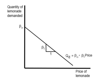
The demand function appearing in equation \ref{d.1.c1} is an example of a linear function. As Figure 1.1 illustrates, the graph of a linear function can be represented as a straight line. [1] As Figure 1.1 illustrates, [latex]\beta _{0}[/latex] is the intercept of this equation on the vertical axis while [latex]\beta _{1}[/latex] is the slope. This slope ([latex]\frac{\Delta \text{Q}_{\text{d}}}{\Delta \text{P}}[/latex]) provides a measure of the change in quantity demanded that results from a one-unit change in the price. Economic theory predicts that the value of [latex]\beta _{1}[/latex] will be negative (since demand curves are expected to be downward sloping). The demand curve illustrated in Figure 1.1 reflects this assumption. Since a demand relationship is only defined for positive values of price and quantity, it is also necessary that [latex]\beta _{o}[/latex] be positive. To determine the relationship between the price of lemonade and the quantity demanded, estimates of the unknown parameters [latex]\beta _{0}[/latex] and [latex]\beta _{1}[/latex] are needed. In equation 1.1, [latex]\beta _{o}[/latex] and [latex]\beta _{1}[/latex] are unknown constants that determine the position of the demand curve. Constants such as these that may represent alternative values are called parameters. As Figure 1.1 illustrates, [latex]\beta _{o}[/latex] is the intercept of this equation on the vertical axis while [latex]\beta _{1}[/latex] is the slope. This slope ([latex]\frac{\Delta \text{Q}_{\text{d}}}{\Delta \text{P}}[/latex]) provides a measure of the change in quantity demanded that results from a one-unit change in the price. Economic theory predicts that the value of [latex]\beta _{1}[/latex] will be negative (since demand curves are expected to be downward sloping). The demand curve illustrated in Figure 1.1 reflects this assumption. Since a demand relationship is only defined for positive values of price and quantity, it is also necessary that [latex]\beta _{o}[/latex] be positive. To determine the relationship between the price of lemonade and the quantity demanded, estimates of the unknown parameters [latex]\beta _{0}[/latex] and [latex]\beta _{1}[/latex] are needed.
Cliometrics
Beginning in the late 1950s, a group of historians and economists began to use econometric tools to analyze historical data. This approach has been referred to as “cliometrics” (in reference to Clios, the muse of history). In 1993, Robert Fogel received the Nobel Prize in economics for his pathbreaking work in this area. Fogel is probably best known for a study of the economics of the U.S. slave system entitled Time on the Cross (coauthored with Stanley Engerman). In Time on the Cross, Fogel and Engerman use an extensive collection of data from plantation records, slave auctions, and the U.S. census to examine the economic functioning of the system of slavery. Other pioneering studies by cliometricians focused on such topics as: the tax burden faced by the U.S. colonies during the colonial period, the effect of the canals and railroads on U.S. economic development, and the causes of the Great Depression.
While there was initially a good deal of controversy over the role of statistical and econometric analysis in historical research, the methodology introduced by Fogel, Engerman, and other cliometricians, has now become an accepted part of a modern historian’s set of research tools.
| Price of lemonade | Quantity sold |
|---|---|
| $0.30 | 46 |
| 0.60 | 43 |
| 0.90 | 35 |
| 1.20 | 31 |
| 1.50 | 32 |
| 1.80 | 30 |
| 2.10 | 23 |
| 2.40 | 17 |
| 2.70 | 13 |
| 3.00 | 10 |
| 3.30 | 9 |
| 3.60 | 3 |
- Economic models typically specify the relationships that exist between a dependent variable and one or more independent variables, holding constant the effect of other variables. Since economists are not generally able to conduct controlled experiments, other variables affect the outcomes. In the case of a demand curve, the quantity of a good demanded at a point in time is affected by factors other than the price of the good. For example, lemonade sales may be affected by the weather, the popularity of the students selling lemonade, and similar factors. (In later chapters we will examine how the effects of other variables can be controlled for through the use of econometric techniques. Even when this is done, however, it is not possible to control for all of the other factors that affect the variable of interest — Q[latex]_{\text{d}}[/latex] in this case.)
- There is an element of randomness in the behavior of individuals. An individual does not always behave in exactly the same way when faced with identical choices. Even when all observable factors are held constant, individuals will sometimes buy more lemonade on some days than on others.
- Economic variables might be incorrectly measured. Errors may occur as a result of inaccurate information provided by individuals or they may result from mistakes in recording the information. Another common source of error in measuring variables is the use of variables that do not directly correspond to the variables specified by economic theory (e.g., econometricians may use test scores such as IQ or SAT scores as imperfect measures of an individual’s “ability”).
- The fitted equation may not reflect the actual functional relationship (e.g., a linear relationship is estimated when the true relationship is nonlinear).
Let’s modify the demand equation to account for these factors. The revised relationship between the observed quantity demanded and the price for observation [latex]i[/latex] can be stated as:
[latex]\text{Q}_{\text{d}i}=\beta _{o}+\beta _{1}\text{Price}_{i}+u_{i} \label{demand} \tag{1.2}[/latex]
\begin{equation*}
\text{where: }u_{i}=\text{random error term for observation}_i.
\end{equation*}[/latex]
The \textbf{random error term} (or disturbance term) in equation 1.2, [latex]u_i[/latex], represents the combination of all factors other than price that affect the quantity of lemonade demanded. This error term includes the effect of all of the factors listed above. It is assumed that the average value of this random error term is zero. Roughly speaking, this assumption means that these errors are just as likely to be positive as negative. (This assumption is discussed in more detail in Chapter \ref{biv.reg.chap}.)
Equation 1.2 is an example of a regression equation. A regression equation provides a relationship between a variable that you are attempting to explain ([latex]Q_{di}[/latex] in this case) and one or more explanatory variables (Price{[latex]_{i}[/latex]} in this example). The variable that you are attempting to explain is called a dependent variable. The dependent variable appears on the left-hand side of the regression equation. The right-hand side of the regression equation contains one or more independent variables} that are assumed to have an effect on the level of the dependent variable. In the demand relationship appearing in equation \ref{demand}, the price of lemonade (Price[latex]_{i}[/latex]) is the only independent variable appearing in the regression equation.
\exbox{Origins of regression analysis}{\indent The term “regression” was first used by Sir Francis Galton in his studies on heredity (Galton, 1899,1908). Galton examined data on the height of parents and their children. He observed that relatively tall parents tended to have children that are taller than average. In a similar manner, parents that were shorter than average generally have children that have below-average height.
Galton noted, however, that the children of tall parents tended to be somewhat shorter than their parents. Similarly, the children of relatively short parents generally tended to be somewhat taller than their parents. Thus, while parent’s height seemed to have a substantial effect on their children’s height, the height of these children tended to drift back to the average height of the population. Galton referred to this tendency as a “regression” towards the population mean. Over time, the term “regression” acquired the more general meaning of a relationship between a dependent variable and a set of independent variables (and a random error term). }
One of the purposes of econometric analysis is to develop a procedure that can be used to estimate the parameters of equations such as the demand relationship appearing in equation \ref{demand}. This estimation procedure is called \textbf{regression analysis}. Regression analysis is one of the most commonly used tools in an econometrician’s toolkit.
\begin{center} \FRAME{ftbpFU}{4.8456in}{3.4731in}{0pt}{\Qcb{Fitted lemonade demand curve}}{% \Qlb{lemon_fit}}{fig1-3.gif}{\special{language “Scientific Word”;type “GRAPHIC”;maintain-aspect-ratio TRUE;display “USEDEF”;valid_file “F”;width 4.8456in;height 3.4731in;depth 0pt;original-width 4.7919in;original-height 3.4272in;cropleft “0”;croptop “1”;cropright “1”;cropbottom “0”;filename ‘graphs/Fig1-3.gif’;file-properties “XNPEU”;}} \end{center}
Figure~\ref{lemon_fit} contains a graph of an estimated demand curve that appears to fit this data fairly well. In this case, the estimated equation is given by:\footnote{% The procedure used to estimate this equation is discussed in Chapter \ref% {biv.reg.chap}.} \begin{equation} \text{\^{Q}}_{\text{d}i}=49.24-38.32\text{Price}_{i} \label{demand1} \end{equation}% In this equation, \^{Q}$_{\text{d}i}$ denotes the value of quantity demanded that is predicted by the estimated regression equation. This predicted value of the dependent variable is often referred to as a \textbf{fitted value}. Throughout this text, fitted or estimated values will be represented by placing a “hat” over the corresponding variable. Thus, for example, \^{Q}$% _{\text{d}i}$ is used to denote the value of quantity demanded that is predicted by the regression equation, while Q$_{\text{d}i}$ is the actual quantity demanded. In a similar manner $\hat{\beta}_{i}$ will be used to denote the estimated value of the parameter $\beta _{i}$.
As Figure~\ref{lemon_fit} indicates, the observed quantity demanded at each price (Q$_{\text{d}i}$) differs from the value predicted by the estimated regression equation (\^{Q}$_{\text{d}i}$) by the observed error term $\hat{u}% _{i}$.\footnote{% The observed error term $\hat{u}_{i}$ will, in general, differ from the true error term, $u_{i}$ because the estimated values of $\beta _{o}$ and $\beta _{1}$ will not, in general, equal the true values of these parameters.} When the observed quantity demanded lies above the curve, $\hat{u}_{i}$ is positive; $\hat{u}_{i}$ is negative when the observed value lies below the estimated curve. Since the average value of $u_{i}$ is assumed to be zero, it seems reasonable to assume that the mean value of the observed error terms ($\hat{u}_{i}$) will also be zero.
A comparison of equations \ref{demand} and \ref{demand1} indicates that the observed error term can also be expressed as the difference between the actual and fitted values of the dependent variable: \begin{equation} \hat{u}_{i}=\text{Q}_{\text{d}i}-\text{\^{Q}}_{\text{d}i} \label{error.1z} \end{equation} Table \ref{dem.er.1} illustrates how the fitted values and the observed error terms may be computed once the regression equation has been computed. The fitted values in the third column of this table are constructed using the results from equation \ref{demand1}.\footnote{% The fitted values have been rounded to the nearest integer.} Once these fitted values are computed, the sample error terms can be easily computed using equation \ref{error.1z}. Note that the average value of the observed error terms is zero. %TCIMACRO{% %\TeXButton{table 2}{\begin{table} %\begin{center} %\begin{tabular}{|c|c|c|c|} \hline %& & $\bf \hat Q_{di}$ & $ \bf \hat u_i$ \\ %\bf{Price} & {$\bf Q_{di}$} & {$\bf =49.2-38P_i$} & {$ \bf =Q_{di} – \hat Q_{di}$} \\ \hline %\$0.10 & 46 & 45 & 1 \\ %0.20 & 43 & 42 & 1 \\ %0.30 & 35 & 38 & -3 \\ %0.40 & 31 & 34 & -3 \\ %0.50 & 32 & 30 & 2 \\ %0.60 & 30 & 26 & 4 \\ %0.70 & 23 & 22 & 1 \\ %0.80 & 17 & 19 & -2 \\ %0.90 & 13 & 15 & -2 \\ %1.00 & 10 & 11 & -1 \\ %1.10 & 9 & 7 & 2 \\ %1.20 & 3 & 3 & 0 \\ \hline %& & average: & 0 \\ \hline %\end{tabular} %\end{center} %\caption{Actual and fitted values: lemonade example.\label{dem.er.1}} %\end{table}}}% %BeginExpansion \begin{table} \begin{center} \begin{tabular}{|c|c|c|c|} \hline & & $\bf \hat Q_{di}$ & $ \bf \hat u_i$ \\ \bf{Price} & {$\bf Q_{di}$} & {$\bf =49.2-38P_i$} & {$ \bf =Q_{di} – \hat Q_{di}$} \\ \hline \$0.10 & 46 & 45 & 1 \\ 0.20 & 43 & 42 & 1 \\ 0.30 & 35 & 38 & -3 \\ 0.40 & 31 & 34 & -3 \\ 0.50 & 32 & 30 & 2 \\ 0.60 & 30 & 26 & 4 \\ 0.70 & 23 & 22 & 1 \\ 0.80 & 17 & 19 & -2 \\ 0.90 & 13 & 15 & -2 \\ 1.00 & 10 & 11 & -1 \\ 1.10 & 9 & 7 & 2 \\ 1.20 & 3 & 3 & 0 \\ \hline & & average: & 0 \\ \hline \end{tabular} \end{center} \caption{Actual and fitted values: lemonade example.\label{dem.er.1}} \end{table}% %EndExpansion
In subsequent chapters, we will examine how regression analysis makes it possible to estimate the slope and intercept terms of equations such as equation \ref{demand} from observed data. Once these parameters are estimated, the results can be used to predict how a dependent variable will change when the level of an independent variable changes. In the example above, the estimated slope of the demand curve is -38.32. This indicates that a \$1 increase in the price of lemonade will cause the quantity of lemonade to fall by approximately 38 glasses each day. A \$0.10 increase in the price of lemonade is expected to cause the quantity of lemonade demanded to fall by approximately 4 glasses each day. The history club can use this information to determine the price that will maximize its profit. (Of course, they must also take into account their costs.)
\subsubsection{Example II: The Keynesian consumption function}
Suppose that Congress is considering a proposal to change either taxes or government expenditure to alter the equilibrium level of GDP. In the Keynesian model of the economy, a small change in the level of spending or taxes can generate a relatively large effect on equilibrium output as a result of the multiplier process. The marginal propensity to consume (MPC) is an important determinant of the magnitude of the multiplier effect.
A simple linear version of the Keynesian consumption function is given by: \begin{equation} \text{C}_{i}=\beta _{o}+\beta _{1}\text{YD}_{i}+u_{i} \label{consumption} \end{equation} \begin{equation*} \begin{array}{ll} \text{where:} & \text{C}_{i}\text{ = real consumption expenditures in year }i% \text{ (billions of chained 1996 dollars)} \\ & \text{YD}_{i}\text{ = real disposable personal income in year }i\text{ (billions of chained 1996 dollars)} \\ & u_{i}\text{ = random error term in year }i \\ & 0<\beta _{1}<1% \end{array}% \end{equation*}
The intercept term in this equation ($\beta _{o}$) is the level of real consumption expenditures that would occur if real disposable income equals zero. The magnitude of the intercept of this function has no practical economic significance since no real-world economy would long survive if it experienced a zero level of disposable personal income. Thus, economic theory generally provides no predictions about the magnitude of the intercept of the consumption function. The intercept of the consumption function is likely to be close to zero, but it may be positive, negative, or zero. While negative levels of consumption have no reasonable economic explanation, neither does a level of real disposable income that is equal to zero. What matters, in practice, is how well the consumption function fits the observed data at observed levels of income.
The slope of the consumption function ($\beta _{1}$) is equal to: \begin{equation} \beta _{1}=\frac{\Delta \text{C}}{\Delta \text{YD}} \label{cons.wrs.1} \end{equation}% This slope coefficient provides a measure of the change in consumer spending that results from a one-unit (\$1) increase in disposable personal income. As noted in virtually all introductory macroeconomics texts, the right-hand side of equation \ref{cons.wrs.1} also serves as the definition of the MPC. Therefore, in equation \ref{consumption}, $\beta _{1}$ equals the MPC . Keynesian theory predicts that $\beta _{1}$ is greater than zero and less than one; it does not tell us what value $\beta _{1}$ actually takes.% \footnote{% In the words of Keynes (1936, p. 96): “The fundamental psychological law, upon which we are entitled to depend with great confidence both \textit{a priori} from our knowledge of human nature and from the detailed facts of experience, is that men are disposed, as a rule and on the average, to increase their consumption as their income increases, but not by as much as their increase in income.”} As in the previous example, a random error term, $u_{i}$, has been added to account for other factors that affect the level of consumption expenditures. Figure~\ref{cons_plot} provides a graph of this relationship.\footnote{% The data used to generate this graph is located in the file “cons.dat” on the disk that accompanies this text.}
\begin{center} \FRAME{ftbpFU}{4.8248in}{4.3535in}{0pt}{\Qcb{Plot of consumption data}}{\Qlb{% cons_plot}}{fig1_4.gif}{\special{language “Scientific Word”;type “GRAPHIC”;maintain-aspect-ratio TRUE;display “USEDEF”;valid_file “F”;width 4.8248in;height 4.3535in;depth 0pt;original-width 4.7712in;original-height 4.3024in;cropleft “0”;croptop “1”;cropright “1”;cropbottom “0”;filename ‘graphs/Fig1_4.gif’;file-properties “XNPEU”;}}
\FRAME{ftbpFU}{5.3272in}{4.3016in}{0pt}{\Qcb{Fitted consumption function}}{% \Qlb{cons_fit}}{fig1_5.gif}{\special{language “Scientific Word”;type “GRAPHIC”;maintain-aspect-ratio TRUE;display “USEDEF”;valid_file “F”;width 5.3272in;height 4.3016in;depth 0pt;original-width 5.271in;original-height 4.2497in;cropleft “0”;croptop “1”;cropright “1”;cropbottom “0”;filename ‘graphs/Fig1_5.gif’;file-properties “XNPEU”;}} \end{center}
To analyze the effect of alternative fiscal policies, we need an estimate of the intercept and slope terms ($\beta _{o}$ and $\beta _{1}$, respectively) in the consumption function above. Figure~\ref{cons_fit} contains a graph of this estimated relationship. Fortunately, econometric analysis provides tools that allow us to estimate the parameters of such equations from observed data on consumption expenditures and disposable income. In this case, the estimated regression equation is: \begin{equation} \text{\^{C}}_{i}=-41.47+0.91\text{YD}_{i} \label{cons.est.c1} \end{equation}% \begin{equation*} \text{(C}_{i}\text{ and YD}_{i}\text{ are expressed in billions of chained 1996 dollars)} \end{equation*}% The estimated slope coefficient in this consumption function, $\hat{\beta}% _{1}$, is 0.91. This suggests that a typical individual will spend \$0.91 out of each additional \$1 of disposable income received.
As these two examples suggest, econometric analysis provides tools that make it possible to relate economic theory to real-world economic processes. Econometrics is also an integral part of economic methodology. Let’s examine the relationship between economic theory and econometric analysis.
\subsection{Hypothesis Testing}
Since economics is a social science, economists rely on the \textbf{% scientific method}. This method suggests that a researcher:
\begin{enumerate} \item observes a phenomena;
\item formulates a hypothesis; and
\item tests the hypothesis. (If the hypothesis is rejected, a new or revised hypothesis must be formulated and tested; if the hypothesis is not rejected, the original hypothesis should be subjected to further testing using new data.) \end{enumerate}
Econometric analysis provides the most common means of testing economic hypotheses. An economic hypothesis generally involves a statement concerning the nature of the relationship between the variable that you are trying to explain and one or more explanatory variables. As in the two examples above, these hypotheses often take the form of a prediction concerning the sign or magnitude of a coefficient in an equation. To illustrate the use of \textbf{% hypothesis tests}, let’s consider a more general form of a demand function for good $X$: \begin{equation} \text{Q}_{\text{d}i}^{x}=\beta _{o}+\beta _{1}\text{P}_{i}^{x}+\beta _{2}% \text{P}_{i}^{y}+\beta _{3}\text{P}_{i}^{z}+\beta _{4}\text{I}_{i}+u_{i} \label{gdemand} \end{equation} \begin{equation*} \begin{array}{ll} \text{where:} & \text{Q}_{\text{d}i}^{x}\text{ = quantity of good }X\text{ demanded at observation }i \\ & \text{P}_{i}^{x}\text{ = price of good }X\text{ at observation }i \\ & \text{P}_{i}^{y}\text{ = price of good }Y\text{ at observation }i \\ & \text{P}_{i}^{z}\text{ = price of good }Z\text{ at observation }i \\ & \text{I}_{i}\text{ = income at observation }i \\ & u_{i}\text{ = random error term for observation }i \\ & i=1,N% \end{array}% \end{equation*} This demand function states that the quantity demanded at each of $N$ observations is assumed to be a linear function of the price of good $X$, the prices of goods $Y$ and $Z$, and income. As in the previous examples, a random error term is included to account for all other factors that may affect the quantity of good $X$ demanded.
The law of demand is nothing more than a hypothesis that states that price and quantity demanded are inversely related, \textit{ceteris paribus}. For the demand function in equation \ref{gdemand}, this hypothesis is equivalent to stating that $\beta _1$ is less than zero. One of the major functions of econometric analysis is to test hypotheses of this sort.
You may also wish to test the hypothesis that $X$ and $Y$ are substitute goods. Two goods are substitutes if an increase in the price of one results in an increase in the quantity of the other good demanded. An inspection of the equation above suggests that goods $X$ and $Y$ are substitutes only if $% \beta _{2}$ is positive. Thus, the hypothesis that $X$ and $Y$ are substitutes is equivalent to a hypothesis that states that $\beta _{2}$ is greater than zero. In a similar manner, the hypothesis that $X$ and $Z$ are complements is equivalent to a hypothesis that states that $\beta _{3}$ is negative. (Two goods are complements if an increase in the price of one results in a reduction in the quantity of the other good demanded.)
The magnitude of the coefficient $\beta _{4}$ provides a measure of the effect of consumer income on the quantity of good $X$ demanded, \textit{% ceteris paribus}. If an increase in income results in an increase in the quantity of good $X$ demanded, then good $X$ is said to be a normal good. A good is an inferior good if an increase in income results in a reduction in quantity demanded. Thus, good $X$ is a normal good if $\beta _{4}$ is positive and is an inferior good if $\beta _{4}$ is negative. Hypothesis tests may be used to help determine whether a good is a normal or inferior good.
The procedures involved in hypothesis tests of this sort are discussed in detail in Chapters \ref{biv.hyp.chap} and \ref{hyp.mult.chap}.
\subsection{Forecasting future outcomes}
Once an econometric model is specified and estimated, the results may be used for forecasting purposes. Consider the estimated demand function for lemonade: \begin{equation*} \text{\^{Q}}_{di}=49.2-38\text{Price}_{i} \end{equation*}
This equation allows the history club to predict the level of lemonade sales that will occur at any level of the price. For example, if they choose to sell lemonade for \$0.55 per glass, it is expected that approximately 28 glasses will be sold. This estimated demand equation allows the organization to predict what its expected sales will be at each possible price.
In the case of the consumption function discussed above, the estimated consumption function allows economic analysts to predict the level of consumption expenditures that will occur at any given level of disposable income. Suppose that a \$10 million increase in disposable personal income is projected for next year. If the estimated MPC is 0.9, then a \$9 million increase in consumption expenditures may be projected.
The usefulness of econometric methods for forecasting purposes is indicated by the widespread use of these techniques by government agencies, independent researchers, consulting firms, and market research firms. Large corporations and utility companies generally have their own forecasting departments that predict the demand for their products. The American Medical Association hires economists to forecast the demand for physicians’ services.
The use of econometric techniques for forecasting purposes will be discussed more extensively in Chapters \ref{biv.reg.chap}, \ref{mult.chap}, and \ref% {ARIMA.chap}.
\section{Formulating an econometric model}
Throughout the remainder of the text, you will examine how econometric models are specified and estimated. To help understand what this process is all about, it will be useful to examine a somewhat more detailed example of the application of econometric analysis. This example should help you understand the relationship between economic theory and econometric analysis.
Suppose an econometrician decides to examine the empirical evidence concerning the quantity theory of money. This theory predicts that an increase in the money supply will primarily result in an increase in the price level. Let’s examine how an economist could test this hypothesis.
\subsection{Model specification}
The first step in conducting an econometric analysis involves the specification of an economic model. This model consists of one or more equations that are assumed to govern the relationships among the economic variables. The demand and consumption functions discussed above are examples of such equations. In this economic model, some variables will be explained by the model while others are assumed to be determined outside of the model. The variables determined within the model are called \textbf{endogenous variables}; the variables determined outside of the model are called \textbf{% exogenous variables}. A useful way of thinking about the distinction between endogenous and exogenous variables is that the endogenous variables in an economic model are the ones that the model is designed to explain; exogenous variables are not explained by the model.
In the demand and supply model, the endogenous variables are the equilibrium price and quantity of the good since both of these variables are simultaneously explained by the model. The exogenous variables in this model are the other variables that affect either the demand or the supply of this good. These exogenous variables include: resource prices, technology, the prices of substitute and complementary goods, consumer income, and similar variables. If any of these factors change, the equilibrium price and quantity will change. These exogenous variables, however, are not explained by the model itself. Instead, they are assumed to be determined outside of the model.
Initially, the focus of this text will be on models in which the dependent variable in a regression equation is the only endogenous variable in the model. The independent variables in these models will be assumed to be exogenous. In practical terms, this means that it will initially be assumed that the independent variables affect the level of the dependent variable, but the dependent variable does not affect the level of the independent variables. In many real-world applications, however, endogenous variables will appear on the right-hand side of a regression equation. Econometric techniques appropriate for the estimation of such equations are discussed in Chapter \ref{simul.chap}.
One of the most difficult tasks facing an econometrician is determining which variables belong in each equation. If you omit variables that are important, the estimated coefficients on the included variables may be partly capturing the effects of the omitted variables. If you include variables that do not belong in the equation, you are estimating unnecessary parameters. The inclusion of irrelevant variables and the exclusion of relevant variables are two types of \textbf{specification error}. The consequences of specification error are discussed in detail in Chapter \ref% {spec.chap}.
In this case, the simple quantity theory of money suggests that a relatively simple relationship exists between the rate of growth in the money supply and the inflation rate. Let’s examine this theory.
\subsection{The simple quantity theory of money}
The simple quantity theory of money is based upon the equation of exchange. This equation is generally stated as:\footnote{% A more detailed discussion of this relationship may be found in virtually any introductory- or intermediate-level macroeconomics text.} \begin{equation} \text{MV}=\text{PY} \label{vel.mon.1} \end{equation} \begin{equation*} \begin{array}{ll} \text{where:} & \text{M = nominal money supply} \\ & \text{V = velocity of money} \\ & \text{P = price level} \\ & \text{Y = real GDP}% \end{array}% \end{equation*} In this relationship, the velocity of money is defined as the number of times that a typical dollar is used to purchase domestically produced final goods and services in a given year. The left-hand side of equation \ref% {vel.mon.1} is a measure of the total dollar value of all money spent on domestically produced final goods and services in a given year. The right-hand side of this equation equals nominal GDP. Thus, as stated above, equation \ref{vel.mon.1} is a tautology — it is true by the definition of velocity.\footnote{% A tautology is a stratement that is true by definition. To see that this equation is a tautology, note that velocity is defined as: \begin{equation*} V=\frac{\text{nominal GDP}}{M}=\frac{PY}{M} \end{equation*}% }
Under the simple quantity theory of money, it is assumed that both velocity and real GDP are constant. If these assumptions are correct, then changes in the money supply will directly affect the price level. In particular, a 10\% increase in the money supply will result in a 10\% increase in the price level in this model. Thus, the quantity theory of money predicts that the inflation rate should equal the rate of growth in the money supply.
To test this hypothesis, a simple linear model may be specified as: \begin{equation} \label{eq.ex.1.a} \text{Inflation rate}=\beta _o+\beta _{1\text{ }}\text{rate of monetary growth}\ +\text{ }u_i \end{equation} Under this specification, the inflation rate is an endogenous variable that is determined by the rate of growth in the money supply. It is assumed that the rate of money growth is an exogenous variable that is determined by the actions of the central monetary authorities (the Federal Reserve Board in the U.S.). Under the simple quantity theory of money, the rate of growth in the money supply is the only variable that affects the inflation rate. Thus, there is only one exogenous variable on the right-hand side of this expression.
The quantity theory of money suggests that the value of $\beta _1$ in equation \ref{eq.ex.1.a} equals one. To test this hypothesis, it is necessary to estimate the parameters of this equation. Before this can be done, you must first collect data on inflation rates and rates of monetary growth. Let’s examine the types of data that may be available for this purpose.
\subsection{Types of Data}
There are four different types of data that may be used to estimate an econometric model:
\begin{enumerate} \item cross-sectional data,
\item time-series data,
\item pooled data, and
\item longitudinal or panel data. \end{enumerate}
\textbf{Cross-sectional data} consists of observations that are measured at a given point in time. The unit of observation may be an individual, a firm, a state, or a country. The U.S. census is an example of a commonly used cross-sectional data set. In the case of the quantity theory of money equation, data on the inflation rates and monetary growth rates in individual countries can be used for estimation purposes. The estimated equation will provide information about the relationship between inflation and money supply growth rates across countries.
\textbf{Time-series data} consists of observations for an individual (or an aggregation of all individuals) that are measured at different points in time. These variables are typically measured on an annual, quarterly, or monthly basis. The relationship between the price level and the money supply in a particular economy may be estimated using time-series observations on these variables. The use of time-series analysis allows you to determine how changes in the money supply relate to changes in the inflation rate over time (in a particular country).
\textbf{Pooled data} involves a mixture of time-series and cross-sectional data. The unit of observation is an individual economic unit at a point in time. Pooled data contains a mix of different economic units measured at different points in time. The relationship between inflation and monetary growth could be estimated using a pooled data set consisting of observations on different countries measured at different points in time.
When pooled data is used, a different collection of observations may be surveyed at different points in time (\textit{e.g.}, different individuals may be surveyed in each time period). \textbf{Panel} (or \textbf{longitudinal% }) \textbf{data} is a type of pooled data in which a cross section of economic units is tracked across time. In most panel-data studies, an initial sample is interviewed in a base-year survey. In subsequent years, follow-up surveys are conducted to gather information from participants in the initial sample. In recent years, panel data studies have received increased attention among applied econometricians.
\subsubsection{Inflation Model}
Suppose that we decide to estimate the relationship between the rate of monetary growth and inflation using cross-sectional data on average annual monetary growth rates and inflation rates for 72 countries during the years 1980 through 1989.\footnote{% Source: World Bank (1991). \textit{World Development Report 1991: The Challenge of Development}. NY: Oxford University Press. Table 13. p. 228. A description of these variables is found in Table \ref{inflat.money.dat} in Appendix \ref{data.appendix}. The data also appears on the data disk accompanying the text in the file “inflation.dat.”} The estimated equation is: \begin{equation} \widehat{\text{Inf}}_{i}=4.859+0.955\text{MGrowth}_{i} \label{mgrowth} \end{equation}
where: INF = average annual inflation rate (1980-1989)
MGROWTH = average annual rate of growth in nominal money supply (percent)
Figure~\ref{inf_reg} contains a plot of the estimated equation (and a scattergram of the actual observations). The estimated value of $\beta _{1}$ (0.955) is quite close to one (the value predicted by the quantity theory of money). Thus, this result appears to be consistent with the simple quantity theory of money. In Chapter~\ref{biv.hyp.chap}, procedures for conducting formal hypothesis tests will be discussed.
\begin{center} \FRAME{ftbpFU}{2.7838in}{4.7962in}{0pt}{\Qcb{Inflation regression}}{\Qlb{% inf_reg}}{fig1-6.gif}{\special{language “Scientific Word”;type “GRAPHIC”;maintain-aspect-ratio TRUE;display “USEDEF”;valid_file “F”;width 2.7838in;height 4.7962in;depth 0pt;original-width 3.6668in;original-height 6.3434in;cropleft “0”;croptop “1”;cropright “1”;cropbottom “0”;filename ‘graphs/Fig1-6.gif’;file-properties “XNPEU”;}} \end{center}
\section{Correlation and Causation}
In evaluating econometric models, it is important to distinguish between \textbf{correlation} and \textbf{causation}. Two variables are correlated if there is a discernible linear relationship between the variables. The variables may be either directly or inversely related. There is a causal relationship between two variables if changes in one variable are a cause of the changes in the other variable. Correlation, however, does not imply causation. If an increase in variable $X$ is associated with an increase in variable $Y$, it is possible that the increase in $Y$ is caused by the increase in $X$. It is also possible that the increase in $X$ is caused by the increase in $Y$. The changes in $X$ and $Y$, however, may be the result of changes in a third variable that affects both $X$ and $Y$.
Suppose, for example, that you estimate the parameters of a linear relationship between the total number of deaths in the U.S. and the number of U.S. secondary school teachers. These estimates are based on annual time-series data for the years 1955 through 1998.\footnote{% The data used to estimate this equation may be found in the file “deaths.dat” on the data disk that accompanies this text.} The estimated equation is: \begin{equation*} \widehat{\text{Deaths}}_{t}=1132.7+0.868\text{Teachers}_{t}\text{(measured in thousands)} \end{equation*}
\begin{center} \FRAME{ftbpF}{2.8288in}{4.7945in}{0pt}{}{\Qlb{mortal_reg}}{fig1-7.gif}{% \special{language “Scientific Word”;type “GRAPHIC”;maintain-aspect-ratio TRUE;display “USEDEF”;valid_file “F”;width 2.8288in;height 4.7945in;depth 0pt;original-width 4.2186in;original-height 7.1771in;cropleft “0”;croptop “1”;cropright “1”;cropbottom “0”;filename ‘graphs/Fig1-7.gif’;file-properties “XNPEU”;}} \end{center}
This equation suggests that when 100 additional high school teachers are employed, approximately 87 additional individuals will die in the population. Figure~\ref{mortal_reg} contains a graph of this relationship. It is somewhat unlikely, however, that the expansion in the number of high school teachers over time is responsible for the increase in the number of deaths. Instead, both variables have increased primarily because of an increase in the size of the population. This illustrates the possibility that an apparent relationship between two variables may be the result of a specification error in which an important explanatory variable is omitted from the equation. %TCIMACRO{% %\TeXButton{Boxed text}{\exbox{The Stock Market and the Super Bowl}{An interesting relationship has been %observed between the outcome of the Super Bowl and the direction of the U.S. stock market. %As noted by Stovall (1988) and others, the stock market generally increases in the years in %which one of the original NFL teams wins the Super Bowl. When one of the %AFC teams wins the Super Bowl, however, the stock market has typically declined over %the course of the year. % %While there appears to be a high correlation between the outcome of the Super Bowl and %performance of the stock market, it is unlikely that the outcome of any Super Bowl %caused a change in the performance of the stock market.}}}% %BeginExpansion \exbox{The Stock Market and the Super Bowl}{An interesting relationship has been observed between the outcome of the Super Bowl and the direction of the U.S. stock market. As noted by Stovall (1988) and others, the stock market generally increases in the years in which one of the original NFL teams wins the Super Bowl. When one of the AFC teams wins the Super Bowl, however, the stock market has typically declined over the course of the year.
While there appears to be a high correlation between the outcome of the Super Bowl and performance of the stock market, it is unlikely that the outcome of any Super Bowl caused a change in the performance of the stock market.}% %EndExpansion
An observed correlation between $X$ and $Y$ may also be the result of chance. William Stanley Jevons believed that he had found evidence that the business cycle was caused by sunspot activity. This sunspot theory of the business cycle is based upon an observed correlation between sunspot activity and the level of output produced. Modern economists do not find this argument convincing. It is likely that this observed correlation is purely coincidental.\footnote{% In a somewhat tongue-in-cheek manner, Sheehan and Grieves (1982) examined the relationship that existed between sunspot activity and the wholesale price index in the U.S. during the years 1889-1978. They found evidence that changes in the U.S. price level had an effect on sunspot activity, but sunspots did not affect the U.S. price level. \par On a somewhat more serious note, the term “sunspot equilibria” has been used in recent years to describe a situation in which equilibrium prices and quantities are affected by expectations based upon the realizations of a random variable that has no other effect on the economy. In these models, a variable such as this is referred to as a “sunspot” variable. Examples of such models may be found in Azariadis (1981) and Woodford (1990).}
The basic problem facing econometricians is that correlations between variables may be observed and measured, but causal relationships can only be inferred from these observations. You can observe that an increase in one variable appears to be associated with an increase in another variable, but you cannot generally observe the causal relationship(s) that exist between these variables. Economic theory, however, often provides hypotheses about the nature of these causal relationships. In constructing econometric models, the best strategy is, when possible, to rely on economic theory to provide assumptions about causal relationships among variables. If the causal relationships that are derived from economic models are invalid, then hypothesis tests should eventually result in the invalidation of the model.
In practice, however, some decisions about model specification cannot be based solely on theoretical grounds. Many economic variables (such as an individual’s ability or motivation) cannot be measured directly and are instead represented by the use of \textbf{proxy variables} that are intended to capture the effect of these unobservable variables. IQ or SAT scores, for example, are often used as proxy variables for an individual’s ability. The choice of specific proxy variables is not generally dictated by economic theory. While economic theory may not always provide a detailed list of variables that should be included in a model, it should always be used to guide the formulation of econometric models.
\section{Overview of Text}
The study of econometrics relies heavily on statistical tools. Chapters \ref% {stat.chap} and \ref{estimators.chap} contain a review of the statistical tools that will be needed throughout the rest of the text. Students who have completed a standard one-semester course in statistics should have already been exposed to most of these concepts.
In Chapter \ref{biv.reg.chap}, the bivariate regression model is introduced more formally. In this chapter, you will examine the process of estimating the parameters of a linear relationship between a dependent variable and a single independent variable. The assumptions of the classical regression model are discussed in this chapter. The use of this model for forecasting purposes is also discussed. The process of hypothesis testing in this model is examined in Chapter \ref{biv.hyp.chap}.
In Chapter \ref{mult.chap}, you will examine the multiple regression model. This model consists of a relationship between a dependent variable and a set of independent variables. Since economic relationships generally involve more than one independent (or explanatory) variables, this model has more general applicability than the bivariate regression model. In this chapter, it is assumed that the ideal conditions of the classical regression model are satisfied. Hypothesis testing in this model is discussed in Chapter~\ref% {hyp.mult.chap}.
A discussion of alternative functional forms appears in Chapters \ref% {linear.chap} and \ref{func.form.ii.chap}. In Chapter \ref{linear.chap}, the linearity assumption is examined. Chapter \ref{func.form.ii.chap} deals with other topics related to functional form. These topics include the effect of rescaling variables, the use of qualitative variables, and the use of simple lag models to describe time series processes. Variables are rescaled when they are measured in different units. For example, data is sometimes expressed in units of 1,000 and is sometimes expressed in units of 1,000,000. Qualitative variables do not represent a specific quantitative value. Instead, these variables represent characteristics that are either present or not present for a particular observation. The presence of a college degree is an example of a qualitative variable. Lag models are used to simplify the estimation of time series models in which the current value of a dependent variable is affected by past values of one or more independent variables.
Chapters \ref{spec.chap} through \ref{het.chap} analyze the implication of violations of the ideal conditions of the classical regression model presented in Chapters \ref{biv.reg.chap} and \ref{mult.chap}. Methods of testing for the presence of each of these violations are discussed. In each case, econometric techniques are discussed that make it possible to correct for the presence of the violation.
In Chapter \ref{limdep.chap}, limited dependent variable models are discussed. The first model discussed is the case of a dichotomous dependent variable. This model is used when you are trying to use observable characteristics to predict the probability that a particular choice will be made. This choice may involve the decision to buy a house, become married, attend college, join a union, or any other binary choice. Alternative techniques for estimating models of this sort are discussed in this chapter. The second type of limited dependent variable model discussed in this chapter is the sample selectivity model. This model is appropriate when the dependent variable is observed only in certain circumstances. For example, you only observe the earnings of individuals who choose to work. We do not know how much an individual who is not working would have earned had he or she decided to work. Those individuals who choose to work may have earnings that differ substantially from the potential earnings that could be received by nonworkers. This induces a potential selectivity bias problem. This problem, and a possible correction technique, is discussed in Chapter \ref% {limdep.chap}.
In Chapter \ref{simul.chap}, simultaneous equation models are discussed. These are economic models in which there is more than one endogenous variable. In this chapter, the two-stage least squares (2SLS) estimation procedure is developed to provide a method of estimating such models..
When working with time-series models, econometricians often examine relationships in which a dependent variable is assumed to be affected by current and past levels of one or more independent variables. For example, it might be reasonable to assume that the current level of consumption expenditures is a function of past as well as current levels of disposable personal income. Chapter \ref{lag.chap} contains a discussion of econometric models of this sort.
It has long been observed that most macroeconomic time series variables tend to exhibit substantial trends over time. While the mean of each of these series may change over time, a long-run equilibrium relationship often appears to exist between two or more of these variables. In recent years, econometrician have developed several econometric models that are designed to represent time series models reflecting these relationships. An introductory discussion of these models is contained in Chapter \ref% {unitroots.chap}.
In many situations, econometricians are able to generate reasonably accurate forecasts of an economic time-series variable using only information about current and past values of the series. The autoregressive integrated moving average (ARIMA) models developed by Box and Jenkins (1976) are particularly useful for this purpose. Chapter \ref{ARIMA.chap} contains a discussion of the Box-Jenkins estimation procedure.
\section{Summary}
In this chapter, we have seen how econometric techniques are used to estimate the magnitude of economic relationships, test hypotheses, and forecast future outcomes. Regression analysis can be used to estimate the parameters of linear equations that govern the relationships among economic variables. The error term in a regression captures the effect of excluded or missing variables, the random behavior of individuals, measurement error, and the selection of incorrect functional forms.
Since economic methodology is based on the scientific method, economic theories must be tested against real-world data. Econometric techniques provide important tools for this purpose. In formulating econometric models, the distinction between correlation and causation should be kept in mind. Economists generally recommend that the specification of an economic model should be based upon economic theory.
\section{Key Concepts}
linear function
parameters
scattergram
random error term
regression equation
dependent variable
independent variable
regression analysis
fitted value
scientific method
hypothesis testing
endogenous variable
exogenous variable
specification error
cross-sectional data
time-series data
pooled data
panel (or longitudinal) data
correlation
causation
proxy variables
\newpage
\section{Exercises and Problems}
\begin{enumerate} \item Explain why the Keynesian consumption function given by: \begin{equation*} \text{C}_{t}=\beta _{o}+\beta _{1}\text{YD}_{t}+u_{t} \end{equation*} contains the error term $u_{t}.$
\item On page \pageref{nonlinear.int.chap}, it was noted that error terms may be partly the result of using a linear model to represent a nonlinear relationship. Illustrate how this may occur using a diagram containing a scattergram of points corresponding to a nonlinear demand curve and a graph of a linear demand curve that appears to provide a good fit to these observations.
\item Suppose that you are trying to examine the effect of an individual’s education upon his or her income. You have cross-sectional data on both income and years of schooling.
\begin{enumerate} \item Which of these variables is the dependent variable? Which is the independent variable?
\item What are some of the other independent variables that might be expected to affect the dependent variable? \end{enumerate}
\item An econometrician wishes to estimate the Keynesian savings function. She has data on both savings and disposable personal income.
\begin{enumerate} \item Which of these variables is the dependent variable? Which\ is the independent variable?
\item Specify a regression function that can be used to represent the Keynesian savings function.
\item What is the economic interpretation of the slope of this savings function. \end{enumerate}
\item Download the spreadsheet version of the \textquotedblleft cons\textquotedblright\ data set from the web site accompanying this text. Use a spreadsheet program to construct a new column containing the predicted value of real consumption expenditures (\^{C}$_{t}$) at each level of disposable income using the formula in equation \ref{cons.est.c1}.
\begin{enumerate} \item Construct a new column that contains the sample error term ($\hat{u}% _{t}=$ C$_{t}-$\^{C}$_{t}$).
\item Is there anything interesting about the magnitude of the error terms during the years 1942-1945? What does the sign of the error term tell you about the relationship between the observed outcome and the value predicted by the regression equation? \textit{\ }Are the observed points during these years above or below the regression line? What happened during this period that might account for this phenomenon?
\item How do the error terms in the years 1993 through 2000 compare to those in other time periods? What does the sign of these error terms tell you about the relationship between predicted and actual consumption levels? Are the observed points above or below the regression line for these observations? \end{enumerate}
\item Locate the most recent 15 years of annual data on real consumption expenditures and real disposable income in the most recent release of the \textit{Economic Report of the President}. (A link to an online version of this report is available on the web site that accompanies this text.)
\begin{enumerate} \item Construct a scatterplot of these 15 observations on a graph in which real consumption expenditures are on the vertical axis and real disposable income is on the horizontal axis. The easiest way to do this is to use a spreadsheet software package or a statistical software package that generates graphical displays. \end{enumerate}
\item Equation \ref{demand1} does not contain an error term. Why might the error term be excluded when you are trying to predict the value of a dependent variable that occurs at a given level of an independent variable? (Hint: what is the most reasonable value to assign to this error term if you are trying to forecast outcomes?
\item An economist uses time-series data to estimate the parameters of the following demand curve for natural gas: \begin{equation*} \text{QD}_{t}^{ng}=\beta _{o}+\beta _{1}\text{P}_{t}^{ng}+\beta _{2}\text{P}% _{t}^{oil}+\beta _{3}\text{P}_{t}^{coal}+\beta _{4}\text{P}_{t}^{elec}+\beta _{5}\text{Temp}_{t}+\beta _{6}\text{Inc}_{t}+u_{t} \end{equation*} \begin{equation*} \begin{array}{lcl} \text{where:} & \text{QD}_{t}^{ng} & \text{= total quantity of natural gas demanded in year }t \\ & \text{P}_{t}^{ng} & \text{= average price of natural gas during year }t \\ & \text{P}_{t}^{oil} & \text{= average price of oil during year }t \\ & \text{P}_{t}^{coal} & \text{= average price of coal during year }t \\ & \text{P}_{t}^{elec} & \text{= average price of electricity during year }t \\ & \text{Temp}_{t} & \text{= average daily temperature in year }t\text{ } \\ & \text{Inc}_{t} & \text{= total household income in year }t% \end{array}% \end{equation*} What signs would you predict for the coefficients $\beta _{1},\beta _{2},\ldots ,\beta _{6}$? Explain.
\item \begin{enumerate} \item In a model of demand and supply, what variables are endogenous?
\item What variables are likely to be exogenous variables in a demand and supply model?
\item In the lemonade example considered in this chapter, is it reasonable to consider the price as exogenous? Under what circumstances would it be endogenous? \end{enumerate}
\item Suppose that you construct a model of the supply and demand for beer.
\begin{enumerate} \item What are the endogenous variables in this model?
\item List some of the exogenous variables that are likely to affect the values of the endogenous variables. \end{enumerate}
\item Equation \ref{consumption} was stated as: \begin{equation*} \text{C}_{i}=\beta _{o}+\beta _{1}\text{YD}_{i}+u_{i} \end{equation*} Is it reasonable to assume that YD$_{i}$ is exogenous in this model? Why or why not?
\item An economist estimates the parameters of a linear regression equation that relates the consumption of automobiles to the price of automobiles using annual time-series data. (The data used for this estimation is contained in Table \ref{car.sales.dat} in Appendix \ref{data.appendix} and in the file entitled “auto.dat” on the data disk.) The estimated equation is: \begin{equation*} \text{\^{Q}}_{t}^{d}=24.34+0.575\text{P}_{t} \end{equation*} \begin{equation*} \begin{array}{ll} \text{where:} & \text{\^{Q}}_{t}^{d}\text{ = index of automotive production in year }t\text{ } \\ & \text{P}_{t}\text{ = index of personal transportation costs in year }t% \end{array}% \end{equation*}
\begin{enumerate} \item Does this refute the law of demand? If not, how can you explain the positive slope coefficient?
\item Are there any other variables that should be included in this equation? If so, list these variables. \end{enumerate}
\item Suppose that you are interested in explaining why unemployment rates differ across different states in the United States. Would time-series or cross-sectional data be most appropriate for such a study? Explain.
\item Suppose that you are interested in determining the effect of an individual’s SAT scores on the rate of growth in his or her earnings over time. What type of data (time series, cross sectional, pooled, or longitudinal) would be most appropriate? Explain.
\item Explain the distinction between correlation and causation.
\item An econometrician estimates that the income elasticity of demand for used cars is 0.75. He claims that he has proven that the demand for used cars is a necessity (since the income elasticity is less than one). Is he correct? Under the scientific method can you ever “prove” that a hypothesis is correct?
\item Can econometric analysis ever be used to prove causation? Explain.
\item Econometricians generally do not observe the quantity or quality of on-the-job training. What variable or variables may be used as proxy variables to capture the effect of investments in on-the-job training on a worker’s earnings? \end{enumerate}
- A careful reader may note that quantity demanded appears on the vertical axis while price appears on the horizontal axis. This differs from the treatment in most economics textbooks (a notable exception is in mathematical economics textbooks, such as Chiang (1984)). The reason for this divergence is that it is customary in mathematical applications to place the dependent variable on the vertical axis while the independent variable is placed on the horizontal axis. Since economists today generally assume that quantity demanded is a function of price, quantity demanded belongs on the vertical axis. Why do most economics texts place price on the vertical axis? This tradition dates back to Alfred Marshall and the early marginalists. In their initial theories of demand, the price that a person was willing to pay is related to the marginal utility received from a good. Since marginal utility is a function of price, the original model of demand suggested that the price that a person is willing to pay for a good is a function of the quantity consumed. Thus, Marshall's textbook (the most popular economics text of its time) placed price on the vertical axis and quantity on the horizontal axis. Most later economics texts followed this tradition.} ↵
