Chapter 7 – Hypothesis Testing in the Mult. Reg. Model
Hypothesis testing in the bivariate regression model was examined in Chapter 5. These hypothesis tests were used to examine hypotheses involving a single parameter. In the current chapter, we will examine how tests of this sort are performed in the multiple regression model. Now that there is more than one variable on the right-hand side of the regression equation, however, more complex hypotheses may be examined. Thus, we can now also examine hypothesis tests that involve sets of regression coefficients.
7.1 The normality assumption
In Chapter 6, no assumptions were made concerning the specific form of the probability density function generating the error terms. It was only assumed that the error terms were independently and identically distributed with a mean of zero and a variance of [latex]\sigma^2[/latex]. Even if we do not know the particular density function generating the error terms, the OLS estimators are BLUE.
It is frequently assumed, however, that the error terms in a regression equation are normally distributed. Under this assumption, each of the [latex]\hat{ \beta}_{j}[/latex] is therefore a linear combination of normally distributed random variables (as a result of the linearity property of the OLS intercept and slope estimators). Thus, this normality assumption implies that the estimated intercept and slope coefficients [latex]\hat{\beta}_{o}, {\beta}_{1},\ldots ,\hat{\beta}_{k}[/latex] are also normally distributed (since any linear combination of normally distributed random variables is also normally distributed).
A variety of central limit theorems, however, indicate that the distribution of the OLS intercept and slope estimators will converge to a normal distribution as the size of the sample increases (assuming that the conditions of the classical regression model are satisfied). Thus, in large samples, the normal density function may appropriately be used for hypothesis tests involving the [latex]\hat{\beta}_{j}[/latex] even if the error terms are not normally distributed.
7.2 Hypothesis tests involving [latex]\beta_j[/latex]
As discussed in Chapter 5, the general procedure for performing hypothesis tests involves the following steps:
- Formulate appropriate null and alternative hypotheses. As noted in Chapter 5, the null hypothesis is often stated as the negation of the relationship that you expect to demonstrate. For example, if you wish to show that a parameter is significantly different than zero, you would select a null hypothesis that states that the true value of the parameter is zero.
- Specify the significance level ([latex]\alpha[/latex]) of the test taking into account the relative costs of Type I and Type II errors. (The cost of Type I and Type II errors were extensively discussed in Chapter 5.
- Determine the distribution of an appropriate test statistic under the null hypothesis.
- Establish the acceptance and rejection regions for this test statistic given the selected significance level.
- Calculate the value of the test statistic and reject the null hypothesis if the test statistic falls in the rejection region.
Let’s examine the process of testing hypotheses involving a single parameter.
7.2.1 The t-ratio
Since each of the estimated intercept and slope coefficients, [latex]\hat{\beta}_j[/latex], is distributed normally with a mean of [latex]\beta_i[/latex](since the OLS estimators are unbiased) and a variance of [latex]\sigma_{\hat{\beta}_i}^2[/latex], the random variable:
[latex]\begin{equation} \tag{7.1} Z=\frac{\hat{\beta}_j-\beta _j}{\sigma _{\hat{\beta}_j}} \end{equation}[/latex]
is distributed as a standard normal variate with a mean of zero and a variance equal to one (as discussed in Chapter 2). In mathematical terms, [latex]Z\sim N(0,1)[/latex].
In virtually all practical applications, however, [latex]\sigma _{\hat{\beta}_{j}}[/latex]is not known a priori. Instead, econometricians must rely on an estimated value of the standard error for these parameters. If the denominator in equation 7.1 is replaced with the estimated standard error for the estimator ([latex]\hat{\sigma}_{\hat{\beta}_{j}}[/latex]), a new variable can be created:
[latex]t=\frac{\hat{\beta}_{j}-\beta_{j}}{\hat{\sigma}_{\hat{\beta}_{j}}}[/latex]
that is distributed according to Student’s [latex]t[/latex]-distribution with [latex]N-(k+1)[/latex] degrees of freedom.[1]
Speed limits and highway fatalities
It is generally assumed that a reduction in the speed limit on interstate highways will save lives. Charles Lave (1985), however, conducted an interesting econometric study that casts some doubt on this argument. In his study, Lave used multiple regression analysis to analyze the determinants of fatality rates on twelve categories of roads. These results suggest that the average speed of vehicles on these highways is less important than the variation in speed in explaining fatality rates. In particular, when other factors were held constant, the [latex]t[/latex]-statistic on the average speed variable in each equation was insignificant at all conventional significance levels.
Lave’s study suggests that fatal accidents are more likely to occur when there is a larger variation in vehicle speed. If all vehicles are traveling at similar speeds accidents are less likely. As Lave states this, “Variance kills, not speed.” (Lave (1985), p. 1159).
7.2.2 Two-tailed tests
Suppose you wish to test whether an intercept or slope parameter is significantly different than a specified value ($=c$). The hypotheses for this test would be: \begin{equation*} \text{H}_{\text{o}}\text{: }\beta _j=c \end{equation*} and \begin{equation*} \text{H}_{\text{1}}\text{: }\beta _j\neq c \end{equation*} To perform a test of this hypothesis, the significance level of the test must be selected. As noted earlier, the significance level is the probability of falsely rejecting the null hypothesis (a Type I error). The most commonly used significance levels are 0.05 and 0.01. In general, a lower significance level should be selected if the cost of a Type I error is relatively high. Choosing a lower significance level, however, results in a higher probability of a Type II error (failing to reject an invalid null hypothesis).
Once the significance level for the test is determined, you must estimate the parameters of the regression equation and the standard errors of the parameter estimates. Using these estimates, a [latex]t[/latex]-statistic can be constructed using the formula:
[latex]\begin{equation}\tag{7.2} t=\frac{\hat{\beta}_{j}-c}{\hat{\sigma}_{\hat{\beta}_{j}}} \end{equation}[/latex]
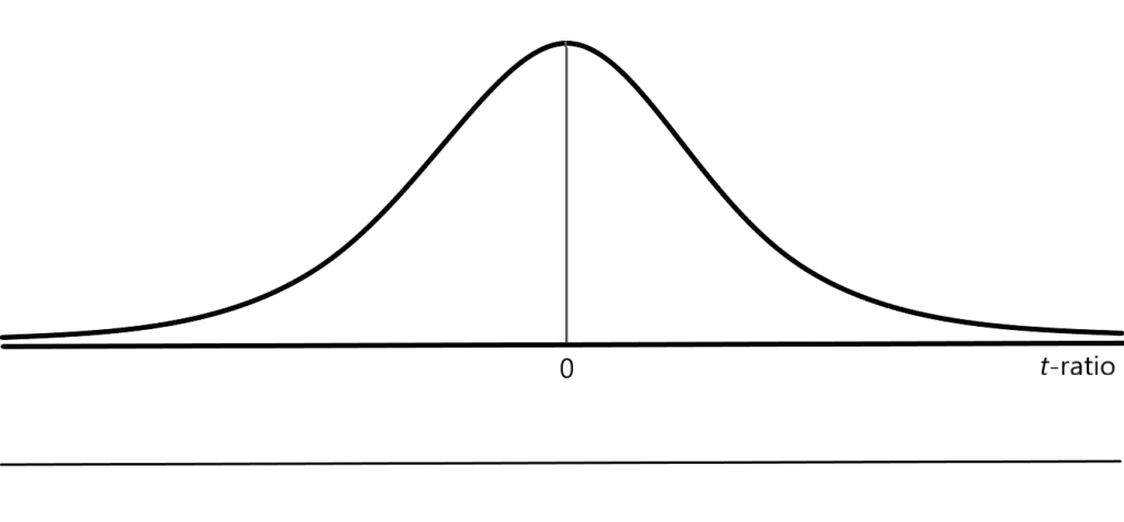
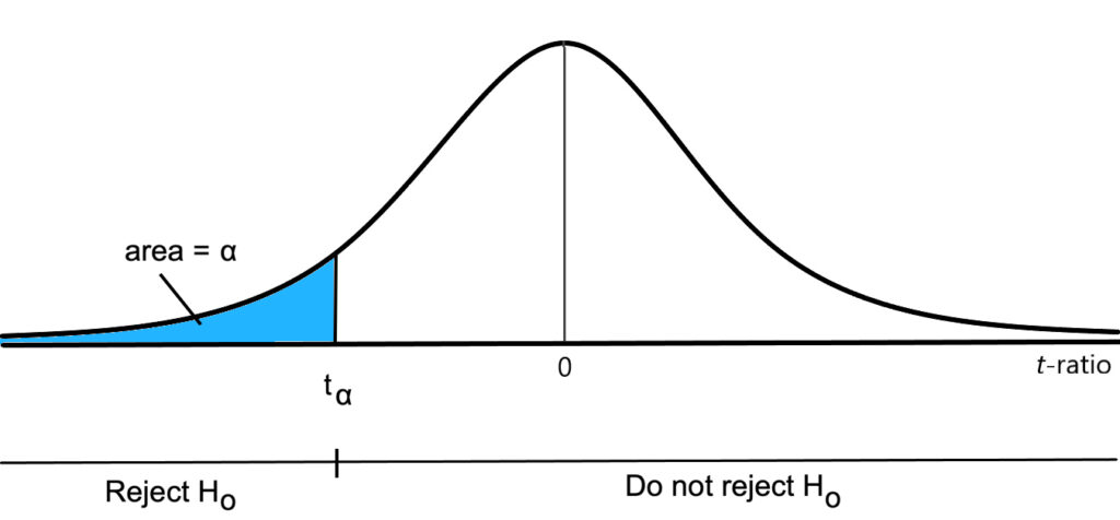
Under the null hypothesis, this ratio is distributed according to Student’s [latex]t[/latex]-distribution with [latex]N-(k+1)[/latex] degrees of freedom. Note that the mean value of the [latex]t[/latex]-ratio is zero if the null hypothesis is correct. The distribution of this statistic (under the null hypothesis) is depicted in Figure 7.1.
To perform a hypothesis test at a significance level of [latex]\alpha[/latex], the acceptance and rejection regions for the test must be determined. Since this is a test to determine whether the parameter is different than a specified value (= [latex]c[/latex]), the null hypothesis can be rejected if the estimated value is either significantly greater than or significantly less than this value. In other words, this is an example of a two-tailed hypothesis test. Critical values of the [latex]t[/latex]-ratio are selected so that the probability of rejecting the null hypothesis equals [latex]\alpha[/latex]. The standard procedure is to select critical values of the [latex]t[/latex]-ratio so that the probability of an outcome in either tail of the distribution equals [latex]\alpha /2[/latex]. These critical values can be found by examining a [latex]t[/latex]-table or a statistical table calculator (for a distribution with [latex]N-(k+1)[/latex] degrees of freedom) and finding the values [latex]t_{\alpha /2}[/latex] and [latex]-t_{\alpha /2}[/latex] so that:
Prob([latex]t>t_{\alpha /2})=\alpha /2[/latex]
and
Prob[latex](t<-t_{\alpha /2})=\alpha /2[/latex]
Since the [latex]t[/latex]-distribution is symmetric, most [latex]t[/latex]-tables (such as the one appearing in Appendix A of this text) will only list the critical values for the positive tail of the distribution.
Once the critical values of the distribution have been determined, a hypothesis test is performed using the following decision rule:
- Reject H[latex]_{o}[/latex] if the estimated [latex]t[/latex]-statistic is less than [latex]-t_{\alpha /2}[/latex] or greater than [latex]t_{\alpha /2}[/latex]. In other words, the rejection criterion is:
reject H[latex]_{o}[/latex] if and only if [latex]\left| t\right| >t_{\alpha /2}[/latex]
- Fail to reject H[latex]_{o}[/latex] if the estimated [latex]t[/latex]-statistic falls between [latex]-t_{\alpha /2}[/latex] and [latex]t_{\alpha /2}[/latex]. Thus, the decision criterion is:
do not reject H[latex]_{o}[/latex] if [latex]\left\vert t\right\vert \leq t_{\alpha /2}[/latex]
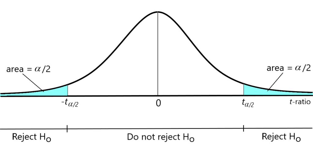
Figure 7.2 illustrates the acceptance and rejection regions for a two-tailed hypothesis test. The shaded area of this diagram equals the probability of rejecting the null hypothesis if the null hypothesis is correct. This area is the probability of a Type I error. Selecting a lower significance level will result in a larger acceptance region and a smaller rejection region.
Automobile Safety Regulation and Deaths
During the mid-1960s the federal government became more actively involved in regulating automotive safety. By the late 1960s, automotive manufacturers were required to provide seat belts for all passengers, an energy-absorbing steering column, a dual braking system, a penetration-resistant windshield, and similar requirements. The purpose of this legislation was to make automotive travel safer for drivers and passengers.
Peltzman (1975) conducted an econometric examination of the effect of these safety improvements on highway death rates. Evidence from both cross-sectional and time-series analyses suggests that these safety improvements did not affect highway death rates. Peltzman suggests that such an outcome is the result of a rational response to improved auto safety. His study suggests that drivers have a greater incentive to drive carefully when there is a higher potential cost associated with reckless driving. When drivers know that they are less likely to be killed in an accident, they have less incentive to drive carefully.
7.2.3 A test of the hypothesis: [latex]\beta_{j}=0[/latex]
As noted in Chapter 5, econometricians are often interested in determining whether a particular independent variable has a significant effect on the dependent variable under analysis. In the multiple regression model, this is equivalent to determining whether a particular slope parameter is significantly different than zero. In other words, if you wish to determine whether the variable [latex]X_i[/latex] has a statistically significant effect on the dependent variable [latex]Y[/latex], this can be examined by testing the hypotheses:
H[latex]_o[/latex]: [latex]\beta_j=0[/latex]
and
H[latex]_1[/latex]: [latex]\beta_j\neq 0[/latex]
If the null hypothesis can be rejected (at the appropriate significance level), then it may be claimed that [latex]X_j[/latex]has a significant effect on [latex]Y[/latex].
When testing to determine whether a particular variable is significantly different than zero, the $t$-ratio once again reduces to:
[latex]\begin{equation} \tag{7.3} t=\frac{\hat{\beta}_j}{\hat{\sigma}_{\hat{\beta}_j}} \end{equation}[/latex]
This type of hypothesis test is so commonly used that virtually all regression analysis software routinely provides a list of the [latex]t[/latex]-ratios defined in equation 7.3 whenever a regression is performed.
Let’s consider some examples of two-tailed hypothesis tests.
7.2.4 Example: The consumption function revisited
In Chapter 6, an expanded version of a consumption function was estimated using U.S. time series data. This estimated consumption function can be written as:[2]
[latex]\begin{equation} \tag{7.4} \text{\^{C}}_{t}=\underset{(10.756)}{-14.476}+\underset{(0.01186)}{0.7468} \text{YD}_{t}+\underset{(0.002187)}{0.03267}\text{Wealth}_{t}-\underset{ (1.9186)}{5.40}\text{Interest}_{t} \end{equation}[/latex]
\begin{equation*} \text{(standard errors in parentheses)} \end{equation*}
Equation 7.4 provides an example of one of the most common ways in which estimated regression equations are expressed: the standard error of each parameter estimate is listed below each estimated coefficient. This equation provides us with all of the information needed to perform hypothesis tests on the individual intercept and slope coefficients.
Let’s suppose that an economist argues that the MPC (marginal propensity to consume) equals one. In equation 7.4, the estimated value of the MPC is given by the parameter [latex]\hat{\beta}_{1}[/latex]. Thus, a test of this hypothesis may be formulated using the following null and alternative hypotheses:
H[latex]_o[/latex]: [latex]\beta_{1}=1[/latex]
and
H[latex]_1[/latex]: [latex]\beta_1\neq 1[/latex]
To test the null hypothesis, a [latex]t[/latex]-statistic must be formulated using equation 7.2:
[latex]\begin{equation}\tag{7.5} t=\frac{\hat{\beta}_{1}-c}{\hat{\sigma}_{\hat{\beta}_{1}}} \end{equation}[/latex]
\begin{equation*} =\frac{0.7468-1}{0.01186} \end{equation*}
\begin{equation*} =-21.35 \end{equation*}
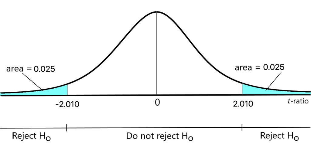
Before testing this hypothesis, a significance level must be selected. Let’s suppose that a 5% significance level is chosen. As noted above, each of the estimated intercept and slope coefficients is distributed as a [latex]t[/latex]-distribution with [latex]N-(k+1)[/latex] degrees of freedom. Since the parameters of this model were estimated using 53 years of annual time series data, the [latex]t[/latex]-ratio given in equation 7.5 is distributed as a [latex]t[/latex]-distribution with 49 degrees of freedom (since the number of slope parameters, [latex]k[/latex], equals three in this model). Using a [latex]t[/latex]-table or a software package that provides critical values for a [latex]t[/latex] distribution, we can easily determine that the critical values for this [latex]t[/latex]-statistic are -2.010 and 2.010. The null hypothesis above should be rejected if and only if the estimated [latex]t[/latex]-ratio is greater than 2.010 or less than -2.010. The acceptance and rejection regions are illustrated in Figure 7.3. (Notice that the total area in the rejection region equals 0.05.)
Since the estimated value of the [latex]t[/latex]-statistic (-21.35) lies within the rejection region, the null hypothesis can be rejected. Thus, this test indicates that the MPC is significantly different than one at a 5% significance level. You should be sure to remember, however, that hypothesis tests of this sort are not infallible. In particular, when a 5% significance level is chosen, a true null hypothesis will be rejected 5% of the time.
The most common form of two-tailed hypothesis test, however, involves testing to determine whether a parameter is significantly different than zero. Let’s suppose that we wished to construct a test to determine whether real disposable income has a significant effect on the level of real consumption spending (holding real wealth and the real interest rate constant). This is equivalent to determining whether [latex]beta_{1}[/latex], the coefficient multiplying YD[latex]_{t}[/latex], is significantly different than zero. Thus, the appropriate hypotheses are:
H[latex]_o[/latex]: [latex]\beta _{1}=0[/latex]
and
H[latex]_1[/latex]: [latex]\beta _{1}\neq 0[/latex]
Using the information from equation 7.4, we can construct the [latex]t[/latex]-ratio as:
\begin{equation*} t=\frac{\hat{\beta}_{1}}{\hat{\sigma}_{\hat{\beta}_{1}}} \end{equation*}
\begin{equation*} =\frac{0.7468}{0.01186} \end{equation*}
\begin{equation*} =62.97 \end{equation*}
Once again, this [latex]t[/latex]-ratio is distributed according to a [latex]t[/latex]-distribution with 49 degrees of freedom. Thus, the critical values equal -2.010 and 2.010 (as depicted in Figure 7.3). Since the estimated [latex]t[/latex]-statistic falls in the rejection region for this hypothesis test, we can reject the null hypothesis and claim that the coefficient [latex]\hat{\beta}_{1}[/latex] is significantly different than zero at the .05 significance level.
Let’s determine whether the other intercept and slope parameters are significantly different than zero. It will be convenient to restate equation 7.4 as:
[latex]\begin{equation} \tag{7.6} \text{\^{C}}_{t}=\underset{(-1.35)}{-14.476}+\underset{(62.97)}{0.7468}\text{YD}_{t}+\underset{(14.94)}{0.03267}\text{Wealth}_{t}-\underset{(-2.81)}{5.40}\text{Interest}_{t} \end{equation}[/latex]
(t-ratios in parentheses)
In equation 7.6, [latex]t[/latex]-ratios have been placed in parentheses below each estimated coefficient. This is another standard method of presenting regression results. Each of these [latex]t[/latex]-ratios can be directly used to test the hypotheses:
H[latex]_o[/latex]: [latex]\beta _{j}=0[/latex]
and
H[latex]_1[/latex]: [latex]\beta_{j}\neq 0[/latex]
In each case, the decision rule is:
Reject H[latex]_o[/latex] if and only if [latex]|t| >t_{\alpha/2}[/latex]
As noted above, the critical values for a [latex]t[/latex]-distribution with 49 degrees of freedom are -2.010 and 2.010 when a 5% significance level is selected. Thus, the decision rule becomes:
Reject H[latex]_o[/latex] if and only if [latex]|t| > 2.010 [/latex]
Since the absolute value of each of the estimated [latex]t[/latex]-ratios for the slope coefficients in equation 7.6 is greater than 2.010, each estimated slope coefficient is significantly different than zero at a 5% significance level. Note that the intercept term is not significantly different than zero at this significance level.
It should be noted that coefficients that are significant at a 5% significance level may not be significant if a 1% significance level is chosen. The critical values for the [latex]t[/latex]-ratio (with 49 degrees of freedom) are -2.68 and 2.68 at a 1% significance level. An inspection of equation 7.6 indicates that, in this case, all of the slope coefficients remain significantly different than zero at a 1% significance level.
A simple [latex]t[/latex] test: [latex]\left| t\right| >2[/latex]
As noted in Chapter 5, the [latex]t[/latex]distribution asymptotically approaches the normal distribution as the size of the sample increases. Thus, in large samples, the critical values of the [latex]t[/latex]-ratio at a .05 significance level approach 1.96 and -1.96 (the critical values under a normal density function). The decision rule in this case is:
Fail to reject H[latex]_o[/latex] if [latex]\left| \frac{\hat{\beta}_j}{\hat{\sigma}_{\hat{\beta}_j}}\right| \leq 1.96[/latex]
Reject H[latex]_o[/latex] if [latex]\left| \frac{\hat{\beta}_j}{\hat{\sigma}_{\hat{\beta}_j}}\right| >1.96[/latex]
Thus, in reasonably large samples (roughly d.f.>60), a simple rule of thumb is to note that if the estimated [latex]t[/latex]-ratio for a regression coefficient is greater than two, the coefficient is significantly different than zero at a 5% significance level.
It should be noted, however, that this rule of thumb is only an approximation. It should not be used in place of a [latex]t[/latex]-table or statistical calculator for conducting hypothesis tests.
7.2.5 P-values
As noted in Chapter 5, many econometrics packages provide a statistic called a p-value. This statistic provides a convenient tool to test whether a regression coefficient is significantly different than zero. The p-value is defined as:[3]}
p-value = Prob[latex](|t| >\left| \frac{\hat{\beta}_{j}}{\hat{\sigma}_{\hat{\beta}_{j}}}\right|[/latex]
The p-value is a measure of the probability of observing a [latex]t[/latex]-ratio that has an absolute value that is greater than or equal to the absolute value of the observed [latex]t[/latex]-ratio. In other words, the p-value provides the estimated probability of committing a type I error by rejecting the null hypothesis (assuming that the null hypothesis is correct). Thus, the p-value is sometimes referred to as the exact significance level of the test.[4]} A regression parameter is significantly different than zero if the p-value associated with the coefficient is less than the selected significance level.
The p-value may also be used to test whether a variable is significantly greater than (or less than) zero. As noted in Chapter 4, the p-value for a one-tailed test equals one-half of the p-value corresponding to a two-tailed test. A variable is significantly greater than (or less than) zero at a significance level of [latex]\alpha[/latex] if:
[latex]\begin{equation*} \frac{1}{2}\times \text{p-value}<\alpha \end{equation*}[/latex]
One advantage of reporting p-values (along with other information about the estimated parameters) is that this provides the reader with an estimate of the probability of a type I error. Readers who wish to furnish their own interpretation of regression output may find it more useful to know the estimated probability of a type I error rather than just information about whether the estimated parameters are significant at a predefined significance level. Stating that the estimated probability of a type I error is 0.065 provides more information than simply stating that a variable is significantly different from zero at a 10% significance level but is not significantly different from zero at a 5% significance level. If the cost of a type I error is relatively low, a p-value of 0.065, for example, might be seen as an acceptable risk.
7.2.6 One-tailed tests
Two-tailed hypothesis tests are primarily used to determine whether a particular regression parameter differs from a specified value (typically zero). In most econometric applications, a two-tailed test is used to examine whether there is a statistically significant relationship between two variables (holding the effect of other variables constant). A two-tailed test is appropriate, however, only when economic theory generates no predictions about the sign or magnitude of a coefficient. In many cases, however, economic models do generate such predictions. For example, microeconomic theory predicts that the slope of a demand curve is negative. Similarly, Keynesian macroeconomics indicates that the MPC is greater than zero and less than one.
As discussed in Chapter 5, one-tailed hypothesis tests are appropriate when economic theory is able to generate predictions about whether a regression parameter is greater than or less than a specified value. Let’s suppose that economic theory predicts that a particular regression parameter, [latex]\beta_j[/latex], is greater than a specific value, [latex]c[/latex]. To test this hypothesis, a null hypothesis is specified that states that [latex]\beta_j[/latex] is less than [latex]c[/latex]. If the null hypothesis is rejected, then it can be claimed that the [latex]\beta_j[/latex]is significantly greater than [latex]c[/latex]. In mathematical terms, the null and alternative hypotheses would be:
H[latex]_o[/latex]: [latex]\beta_j\leq c[/latex]
H[latex]_1[/latex]: [latex]\beta _j>c [/latex]
To test this set of hypotheses, we can once again form the [latex]t[/latex]-ratio:
[latex]\begin{equation}\tag{7.7} t=\frac{\hat{\beta}_j-c}{\hat{\sigma}_{\hat{\beta}_i}} \end{equation}[/latex]
As noted in Chapter 5, to test the null hypothesis, we assume that it holds as an equality, rather than an inequality. If the estimated value of [latex]\beta_j[/latex] is so large that we can reject the null hypothesis that states that [latex]\beta_j[/latex] is equal to [latex]c[/latex], then we can always reject a null hypothesis that states that [latex]\beta_j[/latex] is less than [latex]c[/latex]. If the true value of [latex]\beta_j[/latex] equals [latex]c[/latex], then the [latex]t[/latex]-statistic in equation 7.7 is distributed as a [latex]t[/latex]-distribution with [latex]N-(k+1)[/latex] degrees of freedom.
Since the null hypothesis should be rejected only if the estimated value of \[latex]beta_{j}[/latex] is significantly greater than [latex]c[/latex], the decision rule becomes:
Reject H[latex]_o[/latex] if and only if [latex]t>t_\alpha[/latex]
where t[latex]_\alpha[/latex] is defined so that:
Prob[latex](t>t_\alpha)=\alpha[/latex]
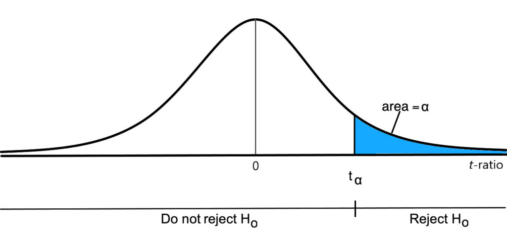
where [latex]\alpha[/latex] equals the significance level of the test. In other words, the critical value of the [latex]t[/latex]-ratio is chosen so that the probability of a Type I error equals [latex]\alpha[/latex] (under the assumption that [latex]\beta_i=c[/latex]).[5] The acceptance and rejection regions for this hypothesis test are depicted in Figure 7.4.
If economic theory instead predicts that a particular regression parameter is less than a particular value ([latex]c[/latex]), a similar procedure is used. A null hypothesis is specified that states that the true parameter value is greater than or equal to this value; the alternative hypothesis states that the true parameter value is less than the specified value. If this null hypothesis can be rejected, then the alternative hypothesis is accepted (at the selected significance level). Thus, the null and alternative hypotheses are:
H[latex]_o[/latex]: [latex]\beta _{j}\geq c[/latex]
and
H[latex]_1[/latex]: [latex]\beta _j < c[/latex]
To test this hypothesis, the [latex]t[/latex]-statistic specified in equation 7.7 is constructed. The acceptance and rejection regions for this test statistic are depicted in Figure 7.5. The null hypothesis is rejected if and only if the estimated [latex]t[/latex]-ratio is less than the critical value [latex]t_\alpha[/latex]. Since this null hypothesis should be rejected only if the estimated value of [latex]\beta _{j}[/latex] is significantly less than the specified value ([latex]c[/latex]), the rejection region lies entirely in the negative tail of the [latex]t[/latex]-distribution.
: A test
In most econometric models, economic theory generates predictions concerning the sign of particular parameters. Thus, the most common form of one-tailed hypothesis test is a test to determine whether a particular parameter is positive or negative. This type of hypothesis test is a special case of the tests discussed above. In this case, the threshold value, [latex]c[/latex], is equal to zero. Thus, the [latex]t[/latex]-ratio reduces to:
[latex]t=\frac{\hat{\beta}_j}{\hat{\sigma}_{\hat{\beta}_j}}[/latex]
Let’s reconsider the estimated consumption function in equation 7.4. Suppose we wished to test the Keynesian hypothesis that states that the MPC is less than one. The appropriate null and alternative hypotheses are:
H[latex]_o[/latex]: [latex]\beta _{1}\geq 1[/latex]
and
H[latex]_1[/latex]: [latex]\beta_1<1 [/latex]
If we wish to test this hypothesis at a 1% significance level, the critical value for a [latex]t[/latex]-distribution with 44 degrees of freedom is -2.4. The estimated [latex]t[/latex]-ratio once again equals:
[latex]t=\frac{\hat{\beta}_{j}-c}{\hat{\sigma}_{\hat{\beta}_{j}}}[/latex]
[latex]=\frac{0.7468-1}{0.01186}[/latex]
[latex]=-21.35[/latex]
Since this falls below the critical value, the null hypothesis can be rejected. Thus, it can be claimed that the estimated MPC is significantly less than one at a 1% significance level.
As noted above, economic theory predicts that consumption expenditures are directly related to the disposable income and wealth and are inversely related to the real interest rate. Thus, economic theory predicts that the[latex]\beta_{1}[/latex]and [latex]beta _{2}[/latex] are both positive while[latex]\beta_{3}[/latex] is negative. Since economic theory generates predictions about the sign of these coefficients, a one-tailed test is appropriate. If a 1% significance level is adopted, the estimated coefficients are significantly greater than zero if the estimated [latex]t[/latex]-ratio is greater than 2.405. An estimated [latex]t[/latex]-ratio of less than -2.405 indicates that the coefficient is significantly less than zero. An inspection of the [latex]t[/latex]-ratios in equation 7.6 indicates that the estimated coefficients multiplying disposable income and real wealth are significantly greater than zero while the estimated coefficient multiplying the real interest rate is significantly less than zero.
7.2.7 Confidence intervals
As discussed in Chapter 5, [latex]t[/latex]-ratios may be used to construct confidence intervals for estimated intercept and slope parameters. A 95% confidence interval for a coefficient can be constructed as:
[latex]\hat{\beta}_j\pm t_{.025}\hat{\sigma}_{\hat{\beta}_j}[/latex]
where [latex]t_{.025}[/latex] is the value of the [latex]t[/latex]-ratio (at the appropriate degrees of freedom) for which 2.5% of the [latex]t[/latex] distribution lies above this value and 2.5% of the distribution lies below [latex]-t_{.025}[/latex]. In repeated samples, confidence intervals constructed in this manner will contain the true parameter value 95% of the time.
More generally, a 100([latex]1-\alpha[/latex] ) percent confidence interval for any intercept or slope coefficient is given by:
100(1-[latex]\alpha[/latex]) percent confidence interval:
[latex]\hat{\beta}_{j}\pm t_{\alpha /2}\hat{\sigma}_{\hat{\beta}_{j}}[/latex]
Returning to the estimated consumption function appearing in equation 7.6, let’s construct a 95% confidence interval for the MPC. The estimated value of the MPC ([latex]\hat{\beta}_{1}[/latex] is 0.7468 and the standard error for this estimator is 0.01186. Since the degrees of freedom of this estimator is 49, the appropriate [latex]t_{.025}[/latex] value is 2.010. Thus a 95% confidence interval for the MPC is given by:
95% confidence interval for the MPC = 0.7468[latex]\pm[/latex]2.010(0.01186)
=0.7468 [latex]\pm[/latex] 0.0238
Therefore, a 95% confidence interval for the MPC includes values between 0.723 and 0.7706.
7.3 Tests involving sets of coefficients
In the multiple regression model, there may be several slope coefficients on the right-hand side of the regression equation. As will be discussed below, it is often desirable to perform tests on sets of these coefficients. Let’s examine these possibilities.
7.3.1 A test of the hypothesis: [latex]\beta_1=\beta _2=...= \beta_k=0[/latex]
All of the hypothesis tests examined up to this point have focused on a single parameter. As will be discussed in Chapter 11, when a multicollinearity problem is present, it is possible that each individual coefficient may be individually insignificant, yet may jointly have a significant impact on the dependent variable. Thus, it would be desirable to have a test that allows us to determine whether the entire set of independent variables exhibits a significant effect on the dependent variable. Fortunately, such a test is available.
Let’s consider the following null and alternative hypotheses:[6]
[latex]\begin{equation}\tag{7.8} \text{H}_{o}\text{: }\beta _{1}=\beta _{2}=...=\beta _{k}=0 \end{equation}[/latex]
and
[latex]\begin{equation*} \text{H}_{1}\text{: at least one slope coefficient, }\beta _{j}\text{, is not equal to }0\text{ } \end{equation*}[/latex]
A relatively simple method of testing this null hypothesis is provided by the use of an [latex]analysis of variance[/latex] (ANOVA) procedure. To understand this procedure, it will be helpful to recall the identity initially discussed in Chapter 4:
[latex]\begin{equation} \tag{7.9} \text{TSS = RSS + ESS} \end{equation}[/latex]
where:
TSS = total sum of squares = [latex]\sum (Y_{i}-\overline{Y})^{2}[/latex]
RSS = regression (explained) sum of squares = [latex]\sum (\hat{Y}_{i}-\overline{Y})^{2}[/latex]
ESS = error sum of squares = [latex]\sum \hat{u}_{i}^{2}[/latex]
Most regression software packages provide printouts that list each of these measures. This information can be used to construct an ANOVA table such as the one appearing in Table 7.1.
| Source | Sum of Squares | d.f. | Mean Sum of Squares |
|---|---|---|---|
| Regression (RSS) | [latex]\sum(Y_i-\overline{Y})^2[/latex] | [latex]k[/latex] | RSS [latex]/ k[/latex] |
| Errors (ESS) | [latex]\sum \hat u_i^2[/latex] | [latex]N-(k+1)[/latex] | ESS [latex]/ N-(k+1)[/latex] |
| Total (TSS) | [latex]\sum(Y_i-\overline{Y})^2[/latex] | [latex]N-1[/latex] |
In addition to each of the components of the total sum of squares, Table 7.1 also lists the corresponding degrees of freedom and mean sum of squares (equal to the sum of squares divided by degrees of freedom). As discussed earlier, the degrees of freedom for a variable is generally equal to the number of observations minus the number of parameters that must be estimated to generate the variable. Since:
\begin{equation*} \hat u_i=Y_i-\hat \beta _o-\hat \beta _1X_{1i}-\ldots -\hat \beta _kX_{ki} \end{equation*}
the estimation of the error sum of squares requires the use of the [latex]k+1[/latex] estimated intercept and slope parameters [latex]\hat \beta _o,\hat \beta _1,\ldots ,\hat \beta _k[/latex]. Thus, the degrees of freedom for the error sum of squares equals [latex]N-(k+1)[/latex]. The degrees of freedom for the total sum of squares equals [latex]N-1[/latex] since the estimation of the total sum of squares requires only one estimated parameter ([latex]\overline{Y}[/latex]). Since the regression sum of squares is the portion of the total variation in [latex]Y[/latex] that is explained by the [latex]k[/latex] independent variables, the degrees of freedom for the regression sum of squares equals [latex]k[/latex].
Once the mean sum of squares are computed, they can be used to construct the following statistic:
[latex]\begin{equation}\tag{7.10} F=\left(\frac{\text{RSS}}{\text{ESS}}\right)\left(\frac{N-(k+1)}{k}\right) \end{equation}[/latex]
Under the null hypothesis [latex]\beta _{1}=\beta _{2}=\cdots =\beta _{k}=0,[/latex] the statistic appearing in equation 7.10 is distributed according to the [latex]F[/latex]-distribution with [latex]k[/latex] and [latex]N-(k+1)[/latex] degrees of freedom.[7] Thus, this statistic may be used to test for the joint significance of all of the slope parameters. In examining the [latex]F[/latex]-statistic in equation 7.10, we can observe that it will be relatively large when the regression equation explains a large proportion of the variance in the dependent variable; the [latex]F[/latex]-statistic will be relatively small, however, when the errors account for most of the variation in the dependent variable. The value of the [latex]F[/latex]-statistic may range anywhere between zero and positive infinity. The [latex]F[/latex]-statistic will equal zero if the independent variables explain none of the variation in the dependent variable; the [latex]F[/latex]-statistic equals infinity only if the error sum of squares equals zero (i.e., only if the regression equation exactly fits all observed data points). Thus, it should be clear that we would reject the null hypothesis given in 7.8 only if the estimated value of the [latex]F[/latex]-statistic falls in the upper tail of the [latex]F[/latex]-distribution. Since the null hypothesis should be rejected only when the [latex]F[/latex]-statistic falls in the upper-tail of the distribution, a one-tailed hypothesis test is appropriate.
This procedure used to test the hypotheses given in 7.8 is quite similar to that used in previous examples of one-tailed hypothesis tests:
- Select a significance level ([latex]=\alpha[/latex]) for the test.
- Determine the acceptance and rejection regions for the test. In this case, this is determined by finding the value of the [latex]F[/latex]-statistic (at the appropriate degrees of freedom) so that the total area lying above this value equals [latex]\alpha[/latex].
- Construct the [latex]F[/latex]-statistic using the definition in equation 7.10.
- Reject the null hypothesis if the estimated $F$-statistic is greater than the critical value.
Let’s consider an example.
7.3.2 Example: The consumption function
Table 7.2 contains analysis of variance information for the estimated consumption function appearing in equation 7.4. Since each of the coefficients is individually significant at the .05 level, we might expect that they should also be jointly significant. In this case, the null hypothesis is:
H[latex]_{o}: \beta _{1}=\beta _{2}=\beta _{3}=0[/latex]
Under the null hypothesis, the statistic:
[latex]\begin{equation} F=\frac{\text{RSS}/k}{\text{ESS}/(N-(k+1))} \tag{7.11} \end{equation}[/latex]
is distributed according to the [latex]F[/latex]-distribution with 3 and 49 degrees of freedom for the numerator and denominator respectively. If we adopt a significance level of .01, we can determine the critical value for the [latex]F[/latex]-test using an [latex]F[/latex]-table (such as the one appearing in Appendix A of this text). For an [latex]F[/latex]-distribution with 3 and 49 degrees of freedom, the critical value of the [latex]F[/latex]-statistic is 4.208.[8] Thus, the decision rule is:
\begin{equation*} \text{Reject H}_{o}\text{ if and only if the }F\text{-statistic is greater than 4.208.} \end{equation*}
Using the information in contained in Table 7.2 the [latex]F[/latex]-statistic can be constructed as:
\begin{equation*} F=\frac{\frac{107,814,694.64}{3}}{\frac{48,433.03}{49}} \end{equation*}
\begin{equation*} =\frac{35,938,231.55}{988.43} \end{equation*}
\begin{equation*} =36358.9 \end{equation*}
Since this [latex]F[/latex]-statistic is greater than the critical value, we can reject the null hypothesis that states that all of the slope coefficients equal zero.
| Source | Sum of Squares | d.f. | Mean Sum of Squares |
|---|---|---|---|
| Regression (RSS) | 107,814,694.64 | 3 | 35,938,231.55 |
| Errors (ESS) | 48,433.03 | 49 | 988.43 |
| Total (TSS) | 107,863,127.67 | 52 |
When multicollinearity is present, it is quite common to find that the whole set of independent variables is jointly significant according to the [latex]F[/latex]-test, even though [latex]t[/latex]-tests of the individual coefficients indicate that the individual coefficients are not statistically significant. Roughly speaking, this situation arises because it is difficult to derive precise estimates of the individual coefficients when there is limited independent variation in the individual independent variables. This possibility is discussed in greater detail in Chapter 11.
7.3.3 R[latex]^2[/latex] and the [latex]F[/latex]-statistic
An interesting relationship exists between the [latex]F[/latex]-statistic discussed above and R[latex]^2.[/latex] Using the definition of the [latex]F[/latex]-statistic contained in equation 7.10:
\begin{equation*} F=\frac{\text{RSS / }k}{\text{ESS / }(N-(k+1) ) } \end{equation*}
\begin{equation*} =\left(\frac{\text{RSS}}{\text{ESS}}\right)\left(\frac{N-(k+1)}{k}\right) \end{equation*}
By equation 7.9, this can be restated as:
\begin{equation*} F=\left( \frac{\text{RSS}}{\text{TSS-RSS}}\right) \left( \frac{N-(k+1)} {k}\right) \end{equation*} \begin{equation*} =\left( \frac{\text{RSS / TSS}}{1\text{-(RSS / TSS)}}\right) \left( \frac{N-(k+1)}{k}\right)\end{equation*}
Using the definition of R[latex]^2[/latex] ( = RSS / TSS), this can be restated as:
\begin{equation} F=\left( \frac{\text{R}^2}{1-\text{R}^2}\right) \left( \frac{N-(k+1)}k\right) \tag{7.12}\end{equation} Thus, if your regression software does not report analysis of variance information, it is possible to compute the [latex]F[/latex]-statistic from the estimated R[latex]^2[/latex] using equation 7.12.
7.3.4 Tests involving linear restrictions on parameters (Wald test)
It is also possible to use an [latex]F[/latex]-test to investigate a wide variety of hypotheses that involve the imposition of one or more linear restrictions on the parameters of a regression equation. A linear restriction is one that can be expressed in the form of a linear equation. Economic theory often places restrictions on the relative size and magnitude of parameters. Consider a regression model given by:
[latex]\begin{equation*} Y_{i}=\beta _{o}+\beta _{1}X_{1i}+\ldots +\beta _{k}X_{ki}+u_{i} \end{equation*}[/latex]
The following are examples of such restrictions:
\begin{equation} \beta _{1}+\beta_{2}=1 \tag{7.13} \end{equation}
\begin{equation} \beta _{3}=\beta_{4.} \tag{7.14} \end{equation}
\begin{equation} \beta _{5}=\beta_{6}=0 \tag{7.15} \end{equation}
The linear restriction appearing in equation 7.13 indicates that the sum of two coefficients add up to one. As will be examined in Chapter 8, tests of hypotheses such as this may be used to examine whether production functions exhibit constant returns to scale. The linear restriction appearing in equation 7.14 indicates that the effect of a one-unit change in [latex]X_3[/latex] will have the same effect on [latex]Y[/latex]as a one-unit change in [latex]X_4[/latex] (holding everything else constant). An application involving a hypothesis test of this sort is discussed below (section 7.3.5). The linear restriction appearing in equation 7.15 indicates that the variables [latex]X_5[/latex] and [latex]X_6[/latex] have no effect on the dependent variable. An example of a test of this sort appears in section 7.3.7 below.
A relatively simple procedure for examining hypotheses such as these is provided by the Wald test.[9] The Wald test essentially involves a choice between two models:
- an unrestricted model in which no restrictions are imposed upon any parameter values, and
- a restricted model that embodies the restrictions captured in the null hypothesis.
Let’s examine how a restricted version of a regression model may be constructed. In Chapter 6, a regression equation was presented that examined the determinants of student success on a microeconomics final exam. The regression relationship was specified as:
\begin{equation} \text{Final}_i=\beta _o+\beta _1\text{SAT-V}_i+\beta _2\text{SAT-M}_i+\beta _3\text{HSGPA}_i+u_i \tag{7.16} \end{equation}
where:
- Final[latex]_i[/latex] = {score received by student [latex]i[/latex] on final exam in introductory microeconomics course
- SAT-V[latex]_i[/latex] = SAT verbal score for student [latex]i[/latex]
- SAT-M[latex]_i[/latex] = SAT math score for student [latex]i[/latex]
- HSGPA[latex]_i[/latex] = cumulative high school grade point average for student [latex]i[/latex]
Suppose that we wished to determine whether SAT verbal and math scores have equal effects on student performance. The null hypothesis for this test is:
\begin{equation} \text{H}_o\text{: }\beta _1=\beta _2 \tag{7.17} \end{equation}
and the alternative hypothesis is:
\begin{equation*} \text{H}_1\text{: }\beta _1\neq \beta _2 \end{equation*}
To test this null hypothesis, we must formulate a restricted version of the regression model. Under the assumption that the null hypothesis is correct, equation 7.17 can be restated as:
\begin{equation} \text{Final}_i=\beta _o+\beta _2\text{SAT-V}_i+\beta _2\text{SAT-M}_i+\beta _3\text{HSGPA}_i+u_i \tag{7.18} \end{equation}
or:
\begin{equation} \text{Final}_i=\beta _o+\beta _2\left( \text{SAT-V}_i+\text{SAT-M}_i\right) +\beta _3\text{HSGPA}_i+u \tag{7.19} \end{equation}
To estimate the restricted version of this model (equation 7.19 ), a new variable must be created that equals the sum of SAT verbal and SAT math scores. Thus, the restricted equation involves only two right-hand side variables: combined SAT scores and high school GPA.
If the restrictions embodied in the null hypothesis (equation 7.17) are correct, then the restricted regression model appearing in equation 7.19 should be able to explain the dependent variable as well as the unrestricted version (equation 7.16)
Let’s examine how a Wald test may be conducted.
The Wald test involves the following procedure:
- Specify a null hypothesis that embodies the linear restriction(s) that you wish to test.
- Select a significance level that is appropriate taking into account the probabilities of Type I and Type II errors.
- Formulate two versions of the regression model: an unrestricted version that does not impose any restrictions on the parameter values; and a restricted version that imposes the restriction(s) on the model before estimation.
- Estimate the parameters of the unrestricted version of the model. Define ESS[latex]_{u}[/latex] as the error sum of squares (= [latex]\sum \hat{u}_{i}^{2}[/latex]) in the unrestricted model.
- Estimate the parameters of the restricted version of the model. Define ESS[latex]_{r}[/latex] as the error sum of squares in the restricted model.
- Formulate the statistic:
\begin{equation} F=\frac{(\text{ESS}_{r}-\text{ ESS}_{u}\text{) / }m}{\text{ESS}_{u}\text{ / }N-(k+1)]} \tag{7.20} \end{equation}
where:
- [latex]m[/latex] = number of linear restrictions
- [latex]N[/latex] = number of observations}
- [latex]k+1[/latex] = number of estimated parameters in the unrestricted model
Under the null hypothesis, this statistic is distributed as an [latex]F[/latex]-statistic with [latex]m[/latex] and [latex]N-(k+1)[/latex] degrees of freedom.[10]
- Determine the critical value of the [latex]F[/latex]-statistic based upon the preselected significance level and define the acceptance and rejection regions for the [latex]F[/latex]-statistic.
- Reject the null hypothesis if and only if the estimated F-statistic is greater than the critical value.
Before discussing specific examples of this procedure, it will be helpful if we examine this test statistic a bit more carefully.
When the unrestricted model is estimated, the parameters are chosen so that the sum of squared residuals is minimized. If a restricted version of this model is estimated, the sum of squared residuals (ESS[latex]_r[/latex]) will always be greater than or equal to the sum of squared residuals in the unrestricted model (ESS[latex]_u)[/latex]. The sum of squared residuals will be equal in the two models only if the restrictions are exactly satisfied in the estimated version of the unrestricted model. Thus, the numerator in equation 7.20, will always be greater than or equal to zero. The numerator will be smaller if the estimated results are consistent with the restriction(s). The numerator will be larger, however, when the unrestricted model fits the data substantially better than the restricted version. Thus, the null hypothesis is rejected only if the [latex]F[/latex] statistic takes on a relatively large value.
Let’s consider a few examples of the application of this procedure.
7.3.5 Example: Student performance on microeconomics final exam
In the previous section, the general procedure for conducting a Wald test was discussed. Let’s conduct a test to determine whether SAT verbal and math scores have equal effects on student performance in an introductory microeconomics course. When the unrestricted version of the model (equation 7.16) is estimated using a sample consisting of 99 observations, the following equation resulted:
\begin{equation} \widehat{\text{Final}}_{i}=-\underset{(-1.68)}{35.366}+\underset{(2.02)}{0.029}\text{SAT-V}_{i}+\underset{(4.25)}{0.058}\text{SAT-M}_{i}+\underset{(1.74)}{0.372}\text{HSGPA}_{i} \tag{7.21} \end{equation}
\begin{equation*} \text{(}t-\text{ratios in parentheses)} \end{equation*}
When the parameters of the restricted model (equation 7.19) are estimated, the sample regression function is:
\begin{equation*} \widehat{\text{Final}_{i}}=-\underset{(20.82)}{29.992}+\underset{(4.62)}{0.044}\left( \text{SAT-V}_{i}+\text{SAT-M}_{i}\right) +\underset{(1.50)}{0.315}\text{HSGPA}_{i} \end{equation*}
\begin{equation*} \text{(}t\text{-statistics in parentheses)} \end{equation*}
| Source | Sum of Squares | d.f. | Mean Sum of Squares |
|---|---|---|---|
| Regression (RSS) | 2,344.16 | 3 | 781.39 |
| Errors (ESS) | 8,779.13 | 95 | 92.41 |
| Total (TSS) | 11,123.29 | 98 |
| Source | Sum of Squares | d.f. | Mean Sum of Squares |
|---|---|---|---|
| Regression (RSS) | 2,155.81 | 2 | 1077.90 |
| Errors (ESS) | 8,967.48 | 96 | 93.41 |
| Total (TSS) | 11,123.29 | 98 |
To form a test of the null hypothesis that states that [latex]\beta _{1}=\beta _{2}[/latex], we can use the analysis of variance information contained in Tables 7.3 and 7.4 to create an [latex]F[/latex]-statistic:
\begin{equation*} F=\frac{(\text{ESS}_{r}-\text{ ESS}_{u}\text{) / }m}{\text{ESS}_{u}\text{ / [ }N-(k+1)]} \end{equation*}
\begin{equation*} =\frac{(8967.48-8779.13)/1}{8779.13/95} \end{equation*}
\begin{equation*} =2.038 \end{equation*}
In this equation, [latex]m[/latex] equals one since a single linear restriction is imposed on the parameters.
If a 5% significance level is selected, the critical value of the [latex]F[/latex]-statistic is approximately 3.95. Since the estimated [latex]F[/latex]-statistic (2.038) is less than this critical value, the null hypothesis cannot be rejected. Thus, we cannot reject the hypothesis that SAT verbal and math scores have an equivalent effect on a student’s performance in a final exam in an introductory microeconomics course.
7.3.6 Tests involving the joint significance of a subset of variables
In many applications, an analyst may wish to test the joint significance of a subset of variables. Suppose, for example, that an econometrician estimates a relationship between an individual’s earnings and a collection of variables that include measures of the individual’s ability, educational attainment, demographic characteristics, and prior work history. The analyst might wish to perform a test to determine whether the set of ability variables is jointly significant. It is quite possible that a set of variables is jointly significant even if individual [latex]t[/latex]-tests indicate that each variable individually is not significantly different than zero.[11]} As will be shown in Chapter 11, this often occurs when an approximate linear relationship exists among the subset of variables (i.e., multicollinearity is present).
If you find that a set of variables is jointly significant, even though the variables are not individually significant, then this indicates that at least one of the variables is significantly different from zero (at the specified significance level). This suggests that at least one of the variables has a significant effect on the dependent variable, but the estimation procedure does not generate sufficiently precise estimates of the individual coefficients to determine which of the variables are important. On the other hand, if you find that a set of variables is jointly insignificant, you may wish to drop the affected variables from subsequent estimates of your model. This should not be done, however, if economic theory indicates that the variables belong in the regression equation. The use of this test for selecting between alternative model specifications is discussed in Chapter 10.
Let’s examine how the Wald test may be used to test of the joint significance of a set of variables.
7.3.7 Example: Presidential election model
In Chapter 6, the voting behavior model appearing in equation 7.22 was discussed.
\begin{equation} \widehat{\text{DVOTE}}_{i}=\underset{(5.40)}{24.272}+\underset{(2.80)}{1.497}\text{un}_{i}+\underset{(4.15)}{0.00145}\text{fedfunds}_{i} \tag{7.27} \end{equation}
\begin{equation*} -\underset{(-0.50)}{1.69}\text{defense}_{i}\text{ + }\underset{(0.22)}{\text{0.00015}}\text{crime}_{i} \end{equation*}
\begin{equation*} \text{(}t\text{-statistics in parentheses)} \end{equation*}
where:
- DVOTE[latex]_{i}[/latex] = proportion of voters selecting the Democratic candidate in state [latex]i[/latex]
- un[latex]_{i}[/latex] = unemployment rate in state [latex]i[/latex]
- fedfunds[latex]_{i}[/latex] per capita federal government spending in state [latex]i[/latex]
- defense[latex]_{i}[/latex] = per capita defense spending in state [latex]i[/latex]
- crime[latex]_{i}[/latex] = total crime rate (crimes per 100,000 population) in state [latex]i[/latex]
An inspection of the [latex]t[/latex]-statistics in equation 7.22 indicates that the “defense[latex]_i[/latex]” and “crime[latex]_i''[/latex] variables are each insignificant at all conventional significance levels. It would be desirable to see if these two coefficients are jointly significant. An appropriate null hypothesis is:
\begin{equation*} \text{H}_o\text{: }\beta _3=\beta _4=0 \end{equation*}
This hypothesis can be tested using the Wald test described above.
First, a restricted form of the regression model must be specified. In this case, however, there are two linear restrictions embodied in the null hypothesis:
\begin{equation*} \beta _{3}=0 \end{equation*}
and
\begin{equation*} \beta _{4}=0 \end{equation*}
| Source | Sum of Squares | d.f. | Mean Sum of Squares |
|---|---|---|---|
| Regression (RSS) | 2086.905 | 4 | 521.738 |
| Errors (ESS) | 1537.783 | 46 | 33.430 |
| Total (TSS) | 3624.688 | 50 |
| Source | Sum of Squares | d.f. | Mean Sum of Squares |
|---|---|---|---|
| Regression (RSS) | 2077.792 | 2 | 1038.896 |
| Errors (ESS) | 1546.897 | 48 | 32.227 |
| Total (TSS) | 3624.688 | 50 |
Imposing these restrictions on the original model results in the following restricted version of the regression model:
\begin{equation*} \text{DVOTE}_{i}=\beta _{o}+\beta _{1}\text{un}_{i}+\beta _{2}\text{fedfunds}_{i}+u_{i} \end{equation*}
When the parameters of this equation are estimated, the sample regression function is:
\begin{equation*} \widehat{\text{DVOTE}}_{i}=\underset{(7.08)}{25.094}+\underset{(2.863)}{1.464}\text{un}_{i}+\underset{(6.93)}{0.00135}\text{fedfunds}_{i} \end{equation*}
\begin{equation*} \text{(}t\text{-statistics in parentheses)} \end{equation*}
\begin{equation*} F=\frac{(\text{ESS}_{r}-\text{ ESS}_{u}\text{) / }m}{\text{ESS}_{u}\text{ / [}N-(k+1)]} \end{equation*}
\begin{equation*} =\frac{(1546.897-1537.783)/2}{1537.783/50} \end{equation*}
\begin{equation*} =0.148 \end{equation*}
Be sure to note that [latex]m[/latex] equals 2 in this case since the null hypothesis imposed two linear restrictions.
If a 5% significance level is adopted, the critical value for this [latex]F[/latex]-statistic (d.f.=2,50) is approximately 3.18. Since the estimated [latex]F[/latex]-statistic falls below this critical value, the null hypothesis cannot be rejected. This means that we cannot reject the hypothesis that states that each of these coefficients is equal to zero. In this case, an econometrician is likely to say that these two variables are jointly insignificant.
7.4 Summary
In this chapter, we have examined how hypothesis testing may be performed in the multiple regression model. In particular, we have examined how to perform tests involving either the magnitude or sign of regression parameters. In summary, the procedure for hypothesis testing involves:
- using an economic model to generate predictions concerning the sign or magnitude of particular coefficients,
- establishing a significance level ([latex]\alpha[/latex]) for the test,
- formulating the null and alternative hypotheses,
- determining the distribution of an appropriate test statistic (such as the [latex]t[/latex]-ratios, [latex]\chi^2[/latex] or [latex]F[/latex]-statistics discussed above) under the null hypothesis,
- establishing the acceptance and rejection regions corresponding to the significance level for the test,
- calculating the value of the test statistic, and
- either rejecting or failing to reject the null hypothesis.
7.4 Key Concepts
- normality assumption
- [latex]t[/latex]-ratio
- hypothesis testing
- type I and type II errors
- significance level
- critical values
- two-tailed test
- one-tailed test
- acceptance region
- rejection region
- p-value
- confidence interval
- analysis of variance
- mean sum of squares
- [latex]F[/latex]-statistic
- Wald test
- restricted model
- unrestricted model
Exercises and problems
- In a classic study of the effect of social security on the level of savings, Martin Feldstein (1974) used annual data for the years 1929 – 1971 (excluding the years 1941-1946) to estimate several versions of a consumption function. One of these estimated equations is given by:
\begin{equation*} \text{\^{C}}_{t}=\underset{(31)}{228}+\underset{(0.047)}{0.530}\text{YD}_{t}+\underset{(0.035)}{0.120}\text{YD}_{t-1}+\underset{(0.074)}{0.356}\text{RE}_{t}+\underset{(0.004)}{0.014}\text{W}_{t-1}+\underset{(0.006)}{0.021}\text{SSW}_{t} \end{equation*}
(standard errors in parentheses)
(all variables are measured in 1958 dollars)
where:
- [latex]\text{\^{C}}_{t}[/latex] = predicted level of real per capita consumption expenditures in year
- YD[latex]_{t}[/latex] = real per capita disposable personal income in year [latex]t[/latex]
- YD[latex]_{t-1}[/latex] = per capita disposable personal income in year [latex]t-1[/latex]
- RE[latex]_{t}[/latex] = real retained earnings (undistributed corporate profit) in year [latex]t[/latex]
- W[latex]_{t-1}[/latex] = real per capita household wealth in year [latex]t-1[/latex]
- SSW[latex]_{t}[/latex] = a measure of the present value of real per capita social security wealth
-
- Economic theory predicts that the signs of each of the above slope coefficients is positive. (No prediction is made concerning the sign of the intercept.) Are one-tailed or two-tailed tests appropriate for the intercept and slope parameters?
- Which of the slope coefficients are significantly different than zero at a .01 significance level? Be sure to state the critical values for the [latex]t[/latex]-statistics. (Note that 36 observations were used to estimate this equation.)
- A market researcher estimates the following sample regression function that predicts the quantity of good [latex]X[/latex] sold in community [latex]i[/latex]
\begin{equation} \widehat{\text{SalesX}}_{i}=\underset{(1.78)}{10.23}-\underset{(-2.45)}{0.37}\text{PriceX}_{i}+\underset{(2.55)}{0.58}\text{PriceY}_{i}+\underset{(1.28)}{0.092}\text{Income}_{i} \tag{7.23} \end{equation}
where:
- SalesX[latex]_{i}[/latex] = per capita annual sales of good [latex]X[/latex] in community [latex]i[/latex]
- PriceX[latex]_{i}[/latex] = price of good [latex]X[/latex] in community [latex]i[/latex]
- PriceY[latex]_{i}[/latex] = price of good [latex]Y[/latex] in community [latex]i[/latex]
- Income[latex]_{i}[/latex] = median income in community [latex]i[/latex]
[latex]t[/latex]-statistics in parentheses)}
using a sample that contains 64 observations.
-
- Which of these parameters are significantly different than zero at a 1% significance level?
- Can you conclude that goods [latex]X[/latex] and [latex]Y[/latex] are substitutes? Conduct a formal test of this hypothesis at a 1% significance level.
- Suppose that an econometrician wishes to test the following null and alternative hypotheses:
H[latex]_o: \beta _3\geq 0[/latex]
and
H[latex]_1:\beta _3<0 [/latex]
using the sample regression function in equation 7.23.
-
- Define the acceptance and rejection regions for this test when a 5% significance level is chosen.
- Can the null hypothesis be rejected in this case?
- Would the null hypothesis be rejected if a 1% significance level had been selected?
- Consider the following model designed to explain the level of life expectancy at birth in different countries: \begin{equation*} \text{LifeEx}_i=\beta _o+\beta _1\text{TV}_i+\beta _2\left( \frac{\text{Pop} }{\text{Doctor}}\right) _i+\beta _3\text{GDP}_i+u_i \end{equation*}
where:
- LifeEx[latex]_i[/latex]= Life expectancy at birth in country [latex]i[/latex]
- TV[latex]_i[/latex] = TV sets per 100 people in country [latex]i[/latex]
- [latex]\left( \frac{\text{Pop}}{\text{Doctor}}\right) _i[/latex] = population per doctor in country [latex]i[/latex]
- GDP[latex]_i[/latex] = real per capita GDP in country [latex]i[/latex] in U.S. dollars
-
- What signs are expected for the slope coefficients?
- Estimate the parameters of this equation using the data in the file “life.dat.”
- Perform a [latex]t[/latex]-test each of the slope coefficients at a 5% significance level. As part of your answer explain whether a one-tailed or two-tailed test is most appropriate in each case.
- At a 5% significance level, perform a test of the null hypothesis given by: H[latex]_o[/latex]: [latex]\beta_1=\beta_2=\beta_3=0[/latex]. Can you reject this null hypothesis?
- Economists use hedonic pricing models to explain price variations in markets in which there is product differentiation. As an example of a hedonic pricing model, consider the following equation describing the determination of new car prices in 2002:
\begin{equation*} \text{MSRP}_{i}=\beta _{o}+\beta _{1}\text{Horse}_{i}+\beta _{2}\text{Length} _{i}+\beta _{3}\text{Width}_{i}+\beta _{4}\text{Height}_{i}+\beta _{5}\text{Weight}_{i} \end{equation*}
\begin{equation*} +\beta _{6}\text{Disp}_{i}+\beta _{7}\text{City}_{i}+\beta _{8}\text{High}_{i}+u_{i} \end{equation*}
where:
- MSRP[latex]_i[/latex] =manufacturer’s suggested retail price for car model [latex]i[/latex] in 2002
- Horse[latex]_{i}[/latex] = horsepower of car model [latex]i[/latex]
- Length[latex]_{i}[/latex] = length of car model [latex]i[/latex] (inches)
- Width[latex]_{i}[/latex] = width of car model [latex]i[/latex] (inches)
- Height[latex]_{i}[/latex] = height of car model [latex]i[/latex] (inches)}
- Weight}[latex]_{i}[/latex] = weight of car model [latex]i[/latex] (pounds)
- Disp[latex]_{i}[/latex] = engine displacement for car model [latex]i[/latex] (liters)
- City[latex]_{i}[/latex] = EPA city miles per gallon for car model [latex]i[/latex]
- High[latex]_{i}[/latex] = EPA highway miles per gallon
- [latex]u_{i}[/latex] = random error term for observation [latex]i[/latex]
-
- For which slope coefficients would a one-tailed test be appropriate? For which slope coefficients would a two-tailed test be appropriate? Explain.
- Use the data in the file “cars.dat” to estimate the parameters of this equation.
- At a 5% significance level, perform the appropriate one-tailed or two-tailed hypothesis test for the slope coefficients in this equation.
- At a 5% significance level, test the joint significance of all of the slope coefficients in this equation.
- Freiden (1974) examined the factors that affect the proportion of women married across states. In this study, 1960 census summary statistics for the 48 contiguous states were used to conduct the empirical analysis. (Freiden also used data on standard metropolitan statistical areas (SMSAs) in this study.) One of the equations estimated by Freiden is:\begin{equation*} \widehat{\text{Married}}_{i}=\underset{(4.20)}{46.45}+\underset{(1.37)}{4.59} \left( \frac{\text{Male earnings}}{\text{Female earnings}}\right) _{i}+ \underset{(1.85)}{13.10}\left( \frac{\text{\# of males}}{\text{\# of females} }\right)_{i} \end{equation*}\begin{equation*} +\underset{(6.67)}{0.137}\text{DivLaws}_{i}-\underset{(-3.02)}{0.501}\text{PropVal}_{i} \end{equation*} \begin{equation*} \text{R}^{2}=0.72 \end{equation*}\begin{equation*} F(4,43)=27.00 \end{equation*}
where
- Married[latex]_{i}[/latex] = proportion of females aged 20-24 married in state [latex]i[/latex]
- [latex]\left( \frac{\text{Male earnings}}{\text{Female earnings}}\right) _{i}[/latex] = ratio of average male earnings to average female earnings
- [latex]\left( \frac{\text{\# of males}}{\text{\# of females}}\right) _{i}[/latex] = ratio of males to females in 20-24 years old age group
- DivLaws[latex]_{i}[/latex]= index measuring the ease of divorce in state [latex]i[/latex]
- PropVal[latex]_{i}[/latex] = median value of owner-occupied housing in state [latex]i[/latex]
(This notation differs from that used in the original study.)
-
- Briefly explain the rationale for including each of these variables.
- Which coefficients are significantly different than zero at a 5% significance level? What is the critical value for the [latex]t[/latex]-statistic?
- Use the [latex]F[/latex]-statistic to conduct a test of the hypothesis: \begin{equation*} \text{H}_{o}\text{: }\beta _{1}=\beta _{2}=\beta _{3}=\beta _{4}=0 \end{equation*} at a 5% significance level.
- (More difficult) Consider the following model of investment demand: \begin{equation} \text{I}_{t}=\beta _{o}+\beta _{1}\text{GDP}_{t}+\beta _{2}\Delta \text{GDP}_{t}+\beta_{3}\text{int}_{t}+u_{t} \tag{7.24}\end{equation}
where:
- I[latex]_{t}[/latex]= real gross private domestic investment in year [latex]t[/latex]
- GDP[latex]_{t}[/latex]= real GDP in year [latex]t[/latex]
- [latex]\Delta[/latex]GDP[latex]_{t}[/latex] =GDP[latex]_{t}[/latex] – GDP[latex]_{t-1}[/latex]
- int[latex]_{t}[/latex] = real interest rate in year [latex]t[/latex]
-
- Discuss why each of the right-hand side variables in this equation may affect the level of investment spending. Can the sign of each variable be predicted using economic theory?
- Use the data appearing in the file “invest.dat” to estimate the parameters of this equation 7.24. Are any of the signs surprising?
- At a 5% significance level, perform an appropriate [latex]t[/latex]-test for each of the slope parameters. Explain whether a one-tailed or a two-tailed test is appropriate in each case.
- A single equation estimation technique is only appropriate when all of the right-hand side variables in the regression equation are exogenous. Is this condition satisfied in this case? Explain.
- Use the definition of the [latex]F[/latex]-statistic in equation 7.10 to show that the value of this statistic will always be greater than or equal to zero.
- If the [latex]F[/latex] statistic in equation 7.10 equals zero, what will be the value of R[latex]^{2}[/latex]?
- Consider the following multiple regression equation designed to explain differences in crime rates across U.S. states: \begin{equation} \text{Crime}_{i}\text{ = }\beta _{o}+\beta _{1}\text{Pov}_{i}+\beta _{2}\text{Metro}_{i}+\beta _{3}\text{Popdens}_{i}+u_{i} \tag{7.25} \end{equation}
where:
- Crime[latex]_{i}[/latex] = total crime rate in state [latex]i[/latex]
- Pov[latex]_{i}[/latex] = poverty rate in state [latex]i[/latex]
- Metro[latex]_{i}[/latex] = metropolitan population as % of state population in state [latex]i[/latex]
- Popdens[latex]_{i}[/latex] = population per square mile in state [latex]i[/latex]
-
- Estimate the parameters of this equation using the data appearing in the file “crime.dat.”
- At a 1% significance level, test to determine whether each of the estimated coefficients has the anticipated sign.
- Use an [latex]F[/latex]-test to test the hypothesis: \begin{equation*} \text{H}_{o}\text{: }\beta _{1}=\beta _{2}=\beta _{3}=0 \end{equation*} at a 5% significance level.
- An econometrician estimates the sample regression function: \begin{equation*} \hat{Y}_{i}=\hat{\beta}_{o}+\hat{\beta}_{1}X_{1i}+\hat{\beta}_{2}X_{2i}+\hat{\beta}_{3}X_{3i} \end{equation*} using a sample consisting of 64 observations. The R[latex]^{2}[/latex] for this equation is 0.624. Use this information to conduct a test of the hypothesis: \begin{equation*} \text{H}_{o}:\beta _{1}=\beta _{2}=\beta _{3}=0 \end{equation*} at a 5% significance level.
- Consider the regression model given by: \begin{equation*} Y_{i}=\beta _{o}+\beta _{1}X_{1i}+\beta _{2}X_{2i}+u_{i} \end{equation*} Suppose that an econometrician wished to test the null hypothesis given by: \begin{equation*} \text{H}_{o}\text{: }\beta _{1}+\beta _{2}=0 \end{equation*} Use this null hypothesis to generate a restricted version of the regression equation (in a form that may be estimated by an OLS estimation procedure).
- Consider the regression model given by: \begin{equation*} Y_{i}=\beta _{o}+\beta _{1}X_{1i}+\beta _{2}X_{2i}+u_{i} \end{equation*} Suppose that an econometrician wished to test the null hypothesis given by: \begin{equation*} \text{H}_{o}\text{: }\beta _{1}+\beta _{2}=1 \end{equation*} Use this null hypothesis to generate a restricted version of the regression equation (in a form that may be estimated using an OLS estimation procedure).
- Suppose that an economist argues that an additional dollar of wealth has the same effect on consumption expenditure as an additional dollar of disposable income. Use the data in the file “cons2.dat” to test the null hypothesis that states that [latex]\beta _{1}[/latex] equals [latex]\beta _{2}[/latex] in the model: \begin{equation*} \text{C}_{t}=\beta _{o}+\beta _{1}\text{YD}_{t}+\beta _{2}\text{Wealth} _{t}+\beta _{3}\text{Interest}_{t}+u_{t} \end{equation*} Use a 5% significance level for this test.
- Use the information in Table 7.3 to construct a Wald test of the null hypothesis: \begin{equation*} \text{H}_{o}:\beta _{1}=\beta _{2}=\beta _{3}=0 \end{equation*} at a 1% significance level. What does the outcome of this test indicate?
- Use the information in Table 7.5 to construct a Wald test of the null hypothesis: \begin{equation*} \text{H}_{o}:\beta _{1}=\beta _{2}=\beta _{3}=\beta _{4}=0 \end{equation*} at a 1% significance level. What does the outcome of this test indicate?
- Consider the following infant mortality model: \begin{equation*} \text{Mortality}_{i}=\beta _{o}+\beta _{1}\text{Calories}_{i}+\beta _{2} \text{HS}_{i}+u_{i}\beta _{3}\left( \text{Pop. / Physician}\right) _{i} \end{equation*} \begin{equation*} +\beta _{4}\left( \text{Pop. / Nurse}\right) _{i}+u_{i} \end{equation*}
where:
- Mortality[latex]_{i}[/latex] = infant mortality rate per 1,000 live births in country [latex]i[/latex]
- Calories[latex]_{i}[/latex] = daily calorie supply per capita in country [latex]i[/latex]
- HS[latex]_{i}[/latex] = % of age group enrolled in secondary education in country [latex]i[/latex] (females)
- [latex]\left( \text{Pop./Physician}\right) _{i}[/latex] = population per physician in country [latex]i[/latex]
- [latex]\left( \text{Pop./Nurse}\right) _{i}[/latex] = population per nursing person in country [latex]i[/latex]
-
- Estimate the parameters of this expanded model using the data in the file “mortal.dat.”
- Are one-tailed or two-tailed hypothesis tests appropriate for each of the slope parameters?
- At a 5% significance level, perform the hypothesis tests selected in part (b). Be sure to state the appropriate critical value as part of your response.
- Use an [latex]F[/latex]-statistic to test the hypothesis: \begin{equation*} \text{H}_{o}\text{: }\beta _{1}=\beta _{2}=\beta _{3}=\beta _{4}=0 \end{equation*} at a 5% significance level. Be sure to state the degrees of freedom and the critical value for your test statistic.
- Consider the infant mortality model appearing in the previous question: \begin{equation*} \text{Mortality}_{i}=\beta _{o}+\beta _{1}\text{Calories}_{i}+\beta _{2}\text{HS}_{i}+u_{i}\beta _{3}\left( \text{Pop. / Physician}\right) _{i} \end{equation*} \begin{equation*} +\beta _{4}\left( \text{Pop. / Nurse}\right) _{i}+u_{i} \end{equation*}
- Mortality[latex]_{i}[/latex] = infant mortality rate per 1,000 live births in country [latex]i[/latex]
- Calories[latex]_{i}[/latex] = daily calorie supply per capita in country [latex]i[/latex]
- HS[latex]_{i}[/latex] = % of age group enrolled in secondary education in country [latex]i[/latex] (females)
- [latex]\left( \text{Pop./Physician}\right) _{i}[/latex] = population per physician in country [latex]i[/latex]
- [latex]\left( \text{Pop./Nurse}\right) _{i}[/latex] = population per nursing person in country [latex]i[/latex]
-
- Estimate the parameters of this model using the data in the file “mortal.dat”
- Are one-tailed or two-tailed hypothesis tests appropriate for each of the slope parameters?
- What are the p-values for each of the estimated coefficients? (Hint: Be sure to take into account whether these are one-tailed or two-tailed tests.)
- Interpret the meaning of each of these p-values.
- Consider the infant mortality model in the previous question. At a 5% significance level, use an [latex]F[/latex]-statistic to test the hypothesis given by: \begin{equation*} \text{H}_{o}\text{: }\beta _{3}=\beta _{4}=0 \end{equation*} State the value of the test statistic, the degrees of freedom and the critical value as part of your answer.
- Estimate the parameters of the voting behavior model given in equation 7.22 using the data in the file “election.dat.” At a 5% significance level, perform a test of the hypothesis: \begin{equation*} \text{H}_{o}\text{: }\beta _{3}=\beta _{4}=0 \end{equation*} Do your results agree with those presented in the text?
- Throughout this text, [latex]k[/latex] is used to represent the number of independent variables in the regression model. Since there are [latex]k[/latex] slope coefficients and 1 intercept coefficient, there are a total of [latex]k+1[/latex] estimated parameters in the regression equation. Thus, the degrees of freedom for the [latex]t[/latex]-statistic equals [latex]N-(k+1)[/latex] since the construction of this statistic requires the estimation of [latex]k+1[/latex] parameters. In some statistics and econometrics texts, [latex]k[/latex] is used to represent the total number of estimated parameters. Under this alternative convention, the degrees of freedom for the [latex]t[/latex]-statistic would equal [latex]N-k[/latex]. The important point to remember, of course, is that the degrees of freedom for the [latex]t[/latex]-statistic will always equal [latex]N[/latex] minus the total number of estimated intercept and slope parameters.} This [latex]t[/latex]-ratio is used to perform hypothesis tests concerning individual regression coefficients in essentially the same manner discussed in Chapter 5. Let's re-examine hypothesis tests of this sort. ↵
- The data used to estimate this equation appears in the file ``cons2.dat.'' ↵
- This is the p-value that it is reported by most regression software packages. It is possible, however, that a regression software package may report the p-value corresponding to a one-tailed test. ↵
- While this terminology is commonly used, the use of the word ``exact'' is somewhat misleading. Since the p-value is derived from sample information, it is an estimate of, and not the actual, probability of a type I error. In this case, the term ``exact'' means only that the p-value provides an estimate of the specific probability of a type I error rather than just information about whether the significance level is less than or greater than a particular threshold (such as 0.05 or 0.01). ↵
- To be more precise, the probability of a Type I error equals [latex]\alpha[/latex] only if the true value of [latex]\beta_{i}[/latex] equals [latex]c[/latex]. If the true value of [latex]\beta_{i}[/latex] is less than [latex]c[/latex], the significance level of the test is less than [latex]\alpha[/latex]. ↵
- Note that only the slope parameters are specified in this null hypothesis. The intercept term is not included among this list of parameters. ↵
- This is a special case of the Wald test discussed below in Chapter 7. The original discussion of this test appears in Wald (1943). ↵
- Since most [latex]F[/latex]-tables appearing in econometric and statistical textbooks (including the F-table contained in Appendix A at the end of this text) do not list the critical value for an [latex]F[/latex]-statistic with 3 and 44 degrees of freedom, the critical value may be obtained either from an econometric software package or from web-based statistical calculators that compute critical values and p-values for a variety of distribution functions. Links to a collection of such calculators may be found on the web site that accompanies this text. ↵
- Wald (1943). ↵
- The proof of this proposition is beyond the scope of this text. A more detailed discussion may be found in more advanced texts. See for example, Greene (2000) pp. 274-6. ↵
- It is also possible, but less likely, that a set of variables may be jointly insignificant even though a [latex]t[/latex]-test would indicate that one or more of the variables is significant. ↵
